Biophysical Chemistry Textbook (Work in Progress)

by John Della Rosa

Introductory Thermodynamics

Introduction

Systems

Defining System and Surroundings

The system refers to the specific portion of the universe that is under consideration for analysis. It is the region or collection of matter and energy that we want to study or focus on. The system is separated from the rest of the universe by an imaginary boundary or surface, which can be real or conceptual.

The surroundings encompass everything external to the system, and they interact with the system. The surroundings include not only the physical environment but also any objects or entities that can exchange energy or matter with the system.

Types of Systems

Open

In an open system, both matter and energy can be exchanged with the surroundings. For example, an open pot of boiling water allows water vapor (matter) and heat (energy) to flow in and out.

Closed

A closed system allows the exchange of energy (usually in the form of heat and work) with the surroundings but does not permit the transfer of matter across its boundaries. A closed container of gas is an example of a closed system.

Isolated

An isolated system does not exchange matter or energy with the surroundings.

State Functions and System Properties

One of the fundamental concepts in thermodynamics is that of state functions. State functions are properties of a system that depend only on the current state of the system and not on the path it took to reach that state. In this chapter, we will list some of the most common state functions or variables that we will encounter.

State Functions

The primary advantage of state functions is that they are independent of the path taken to reach a particular state. Whether a system undergoes a simple or complex process, the change in a state function depends only on the initial and final states, not on the specific steps or intermediate states involved in the process. This makes it much easier to analyze and compare different thermodynamic processes.

It's important to note that not all properties in thermodynamics are state functions. Some variables, known as path-dependent or process-dependent variables, depend on the specific path taken during a process. Examples of path-dependent variables include the amount of heat transferred (Q) and the work done (W) during a process. These variables can vary depending on the specific details of the process and are not uniquely determined by the initial and final states.

Pressure

The force per unit area exerted by a gas on its surroundings. When calculating work, this can be the pressure that the gas must push against in order to expand, rather than the pressure of the gas. This nuance is most important when dealing with irreversible processes, such as adiabatic free expansion.

Volume

The amount of space occupied by a system.

Temperature

A measure of the average kinetic energy of particles in a system.

Laws of Thermodynamics

First Law of Thermodynamics

The first law can be formulated in different ways. A common source of confusion for students is the seemingly inconsistent formula.

Variant 1: $$\Delta U=q+w$$ Variant 2: $$\Delta U=q-w$$ So why will you see both? This is due to differences between authors in how they define the quantities in the equation. Let's start by defining q, which we will call "heat," since this is less controversial. q will be the heat added to the system. Heat flowing (positive q) into the system will increase the amount of internal energy intuitively, so a positive q will contribute to an increase in energy. Heat flowing out of the system (negative q) will decrease the amount of internal energy.

Now, for defining w, which is the "work" term. Here are the two equations again with their definition

$\Delta E=q+w$, positive w here is defined as work done to the system and negative w is defined as work done by the system
$\Delta E=q-w$, positive w here is defined as work done by the system and negative w is defined as work done to the system

Regardless of your definition of w, if work is being performed on the system, energy is being transferred to it, but if the system is expending energy to do work, then it will lose energy. From here on out, the textbook will use variant 1.

Now, the terms work and heat have not been preicsely defined yet. Working definitions for the terms at this point will be:

Work is controlled, harnessed transfer of energy
Heat is uncontrolled transfer of energy

Work can take various forms, but the ones we will be considering will be

Expansion work or "pV work," such as a piston moving due to a pressure difference.
Chemical work, which harnesses energy from chemical reactions

There is a differential form of the equation which is expressed as: $$dE=\delta q + \delta w$$ The heat and work variables have $\delta$ instead because they are inexact differentials. That is to say, they have path-dependent integration. While the change in energy will be the same, the contribution from work vs heat depends on how the process is done.

Second Law of Thermodynamics

The second law of thermodynamics states that total entropy is non-decreasing over time. $$\Delta S_{universe}\geq 0$$ This is sometimes put into formula by breaking down the universe into the "system" or thing of interest and the "surroundings" or everything else. $$\Delta S_{sys}+\Delta S_{surr} \geq 0$$ A common mistake that students make is interpreting it as saying that entropy cannot decrease locally. This is not true. Entropy can very well decrease in a system, but it will be offset by a greater increase in the surroundings. In fact, much of biology involves this very trade-off.

Entropy

What sort of chemical processes have positive $\Delta S$? In general, going from solid to liquid or liquid to gas has an increase in entropy. Creating more molecules from a complex one has positive entropy.

Energy

Forms of Energy

Energy can take different forms. The two main categories are Kinetic and Potential energy. As its name suggests, kinetic energy is associated with movement. Here are 3 forms which we will consider throughout the book:

Translational: a molecule's movement through space
Rotational: a molecule rotating about some axis
Vibrational: bonded atoms vibrating

Potential energy is associated with position rather than movement. This can also take several forms, including but not limited to:

Chemical bonds
Gravitational
Concentration gradients
Electrostatic interactions
Compressed spring

Physics Equations

As one formulation of the First Law states, there is conservation of energy with no input or removal from the system. However, energy can be converted from one form to another. Imagine a ball rolling off of a table; its gravitational potential energy gets converted into kinetic energy, sending it downward. U sometimes refers to potential energy, but also internal energy in general. In this section, U will refer to Potential energy and E will refer to Total energy.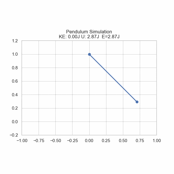

Pendulum Conservation of Energy Simulation

import numpy as np
from scipy.integrate import odeint
import matplotlib.pyplot as plt
import matplotlib.animation as animation
import seaborn as sns
%matplotlib notebook
sns.set_theme(style='whitegrid')

def pendulum(y, t, g, l):
    theta, omega = y
    dydt = [omega, -g/l * np.sin(theta)]
    return dydt

# Initial conditions
theta0 = np.pi/4  # initial angle of displacement
omega0 = 0.0  # initial angular velocity

# Parameters
g = 9.81  # acceleration due to gravity, m/s^2
l = 1.0  # length of the pendulum, m
print(2*np.pi*np.sqrt(l/g))
# Time grid for integration
t = np.linspace(0, 2.1, 150)

# Solve the ODE
sol = odeint(pendulum, [theta0, omega0], t, args=(g, l))

# Set up the figure and axis
fig, ax = plt.subplots(figsize=(6,6))
ax.set_xlim(-1, 1)
ax.set_ylim(-.2, 0.2+l)
ax.set_aspect('equal', 'box')
line, = ax.plot([], [], 'o-', lw=2)
# energy_text = ax.text(0.02, 0.95, '', transform=ax.transAxes)

def init():
    line.set_data([], [])
    energy_text.set_text('')
    return (line, energy_text)

speed_multiplier = 1
def animate(i):
    i*=speed_multiplier
    x = [0, l*np.sin(sol[i, 0])]
    y = [l, -l*np.cos(sol[i, 0])+l]
    
    # Calculate the energies
    h = l - l*np.cos(sol[i, 0])  # height
    v = l * sol[i, 1]  # speed, the derivative of l*theta with respect to time is l*omega
    gpe = g * h  # gravitational potential energy per unit mass
    ke = 0.5 * v**2  # kinetic energy per unit mass
    
    # Update the line and the text
    line.set_data(x, y)
    plt.title('Pendulum Simulation\nKE: {:.2f}J U: {:.2f}J  E={:.2f}J'.format(ke, gpe, gpe+ke))
    
    return (line, energy_text)

ani = animation.FuncAnimation(fig, animate, init_func=init, frames=len(t)//speed_multiplier, interval=10, blit=True)
ani.save('Pendulum-Conservation-of-Energy.gif', fps=60, 
            #extra_args=['-vcodec', 'libx264']
            )
plt.show()

In this section, positive work will refer to work done by the system which is opposite what we had before, but it is common convention. $$W=-\Delta U$$ How is are work required and potential energy related to forces? $$W=\int F\cdot dx$$ The work done is the integral of the force, F, applied over the distance. This force may be a function of the position, x.

Hooke's Law

Hooke's law describes the restoring force in a spring. In plain English, Hooke's law states that the restoring force a spring has is proportional to the displacement from the rest length. $$F=-k(x-x_0)$$ where x is the length of the spring, $x_0$ is the rest length of the spring, k is the spring constant, and F is the force. The sign is negative as the force counteracts the stretching and applies a force in the opposite direction. We can also call $x-x_0$ to be simply x by having our coordinate system have x_0=0; longer is positive x; compressed is negative x. Using our formula for work, we can calculate the work required to stretch a spring. $$W=\int_0^z (-k x) \cdot dx$$ Because the force is in the opposite direction as the dx vector, we get an additional negative sign which cancels things out. $$W=\int_0^z(kx)dx$$ $$=\frac{1}{2}kz^2$$ The work required is $\frac{1}{2}kz^2$ which will be converted into potential energy.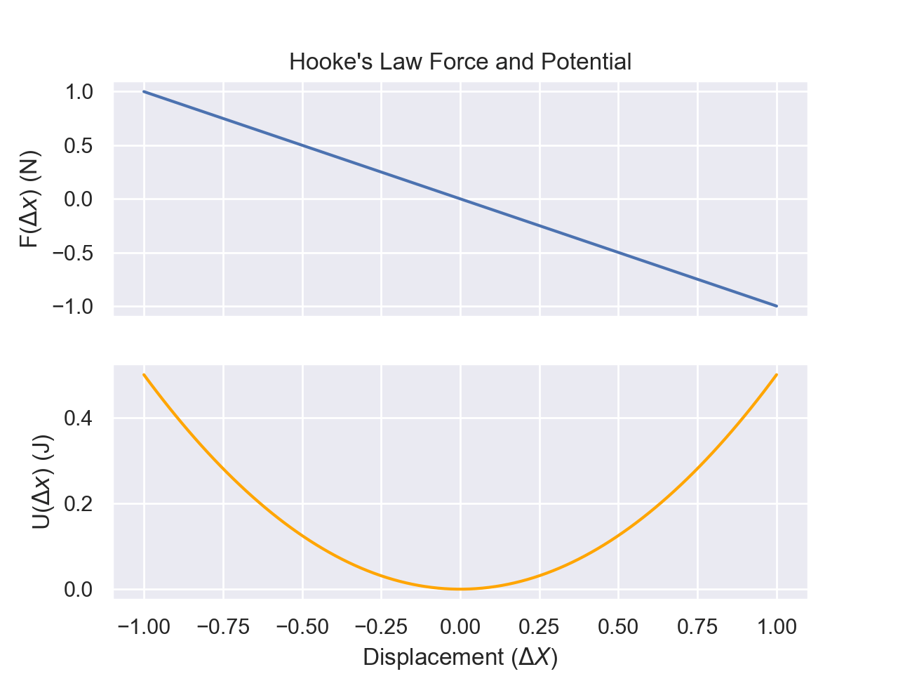

def Hooke_F(delta_x,k):
    return -k*delta_x
def Hooke_U(delta_x,k):
    return 0.5*k*delta_x**2

x_values = np.linspace(-1,1,100)
k=1

fig, axes = plt.subplots(2,sharex=True)

axes[0].plot(x_values,
            [Hooke_F(x,k) for x in x_values])
axes[0].set_ylabel('F($\Delta x$) (N)')

axes[1].plot(x_values,
            [Hooke_U(x,k) for x in x_values],
            color='orange')
axes[0].set_title("Hooke's Law Force and Potential")

axes[1].set_xlabel('Displacement ($\Delta X$)')
axes[1].set_ylabel('U($\Delta x$) (J)')
plt.show()

Electrostatics

Another common force is electrostatic. The electrostatic force between two point charges is described by Coulomb's Law. $$F=\frac{1}{4\pi D\varepsilon_0}\frac{q_1q_2}{r^2}$$ where F is the force, D is the dielectric constant for the medium, $\varepsilon_0$ is the vacuum permittivity (a constant), $q_i$ is the charge of particle i, and r is the distance between the two charged particles. In this form of Coulomb's Law, a negative value for F means an attractive force and a positive F means a repulsive force.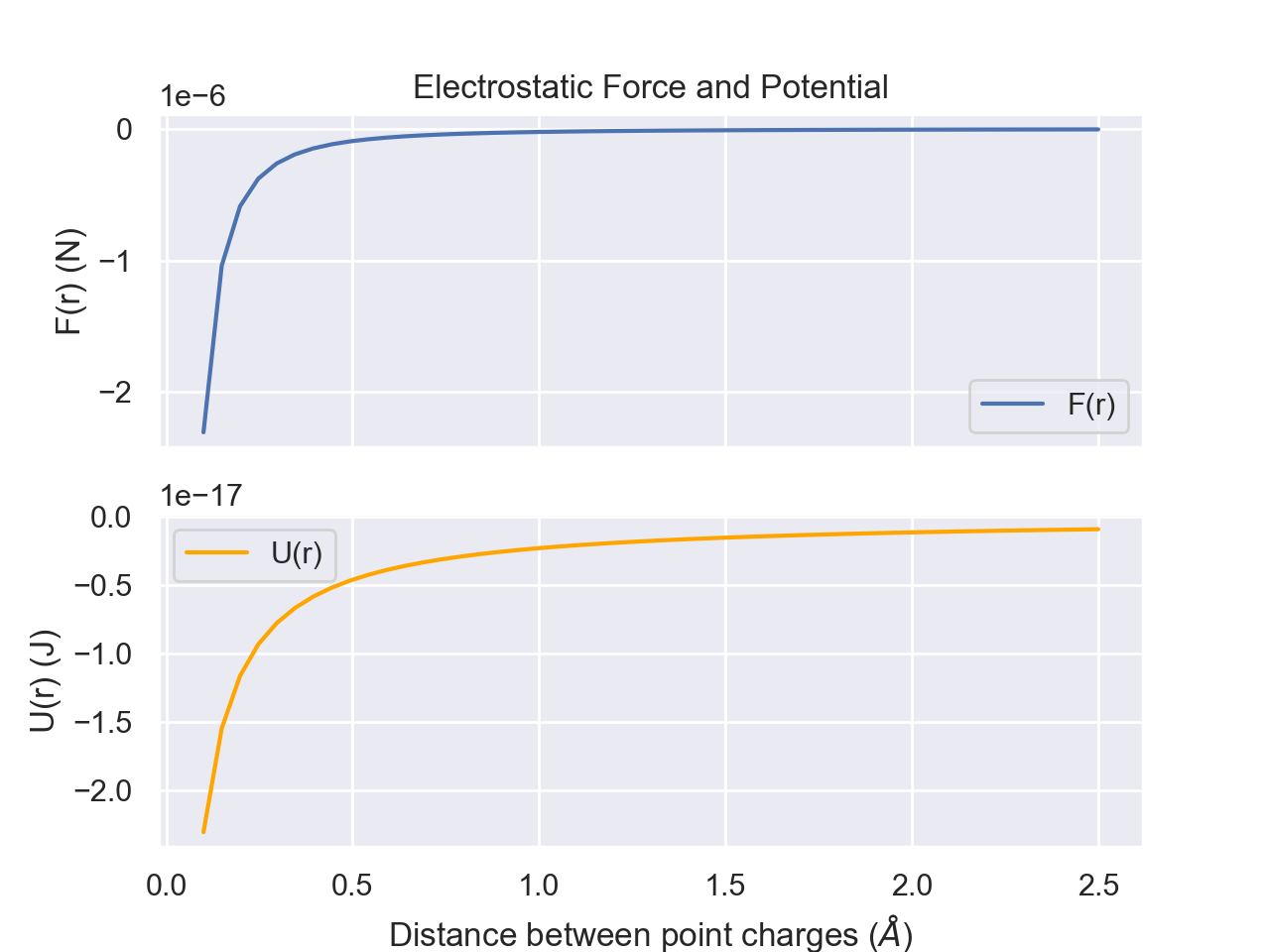

k = 8.98e9

def Coulomb_F(q_1,q_2,r):
    return -k*q_1*q_2/((r*1e-10)**2)
def Coulomb_U(q,Q,r):
    return k*q*Q/(r*1e-10)

x_values = np.linspace(1e-1,1)
q_1 = 1.602e-19
q_2 = -1.602e-19

fig, axes = plt.subplots(2,sharex=True)

axes[0].plot(x_values,
            [Coulomb_F(q_1,q_2,x) for x in x_values],label='F(r)')
axes[0].set_ylabel('F(r) (N)')

axes[1].plot(x_values,
            [Coulomb_U(q_1,q_2,x) for x in x_values],
            color='orange',label='U(r)')
axes[0].set_title("Electrostatic Force and Potential")
axes[0].legend()
axes[1].legend()
axes[1].set_xlabel('Distance between point charges ($\AA$)')
axes[1].set_ylabel('U(r) (J)')
plt.show()

Dielectric constant

The values it can take are $$D \geq 1$$ In a vacuum, D=1. In other mediums, D>1 which makes the electrostatic force weaker. In water, $D_w\approx 80$ which significantly weakens the force. Since much of biology occurs in aqueous environments, this is important to consider. In the interior of proteins, the dieletric constant is much closer to 1, meaning electrostatic interactions on the inside of proteins are stronger than on the outside surface, everything else being equal.

Morse Potential

The harmonic oscillator/Hooke's law model is treating a molecule as if it were two nuclei connected by a spring in a classical sense.

This model is pretty decent at describing behavior close to the equilibrium bond distance, but as r gets further away from $r_e$, we need a better model. This is where the Morse potential comes in. This is an improved version which takes into account things like nuclear-nuclear repulsion from Pauli's exclusion principle and bond dissociation. When r is too small, the Morse potential jumps in potential energy quicker than with a simple Hooke's law approximation. Bonds can't stretch infinitely; bonds break if separation grows too large. The Morse potential takes this into account by having U asymptotically approach a value in the limit as r goes to infinity instead of continuing to increase quadratically. The limit as r approaches infinity is your bond dissociation energy. The equation for the morse potential is given by $$U(r)=D_e (1-e^{-a(r-r_e)})^2-D_e$$ where $D_e$ is related to the dissociation energy.

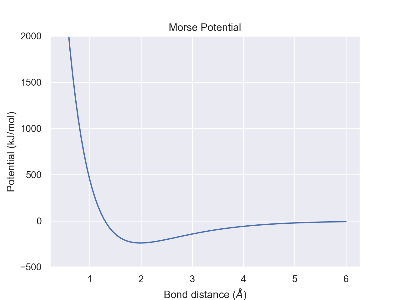
def Morse_U(r,De,a,r_e):
    r = r*1e-10 # convert to angstrom
    r_e = r_e*1e-10
    return De*((1-np.exp(-a*(r-r_e)))**2)-De

x_values = np.linspace(0.3,6,100)
r_e = 1.99
D_e = 240
a = 0.75e10

fig = plt.figure()

plt.plot(x_values,
            [Morse_U(x,D_e,a,r_e) for x in x_values],
            label='F(r)')
plt.ylabel('Potential (kJ/mol)')
plt.xlabel('Bond distance ($\AA$)')
plt.title("Morse Potential")

plt.show()

Lennard-Jones Potential

The Lennard-Jones potential describes Van der Waals interactions between two molecules. The potential is given by $$U(r)=4\varepsilon \left[(\frac{\sigma}{r})^{12}-(\frac{\sigma}{r})^6\right]$$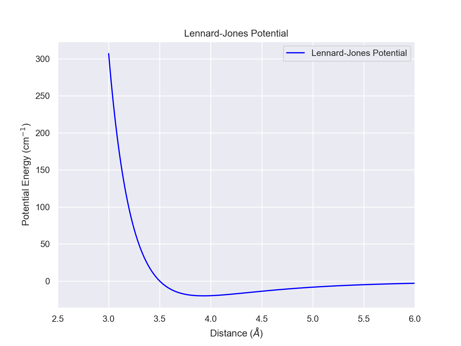

# Constants
epsilon = 20  # Depth of potential well
sigma = 3.5    # Distance at which potential is zero

# Define a range of distances (r)
r = np.linspace(3, 6, 500)

# Calculate the Lennard-Jones potential for each distance
V = 4 * epsilon * ((sigma / r)**12 - (sigma / r)**6)

# Create the plot
plt.figure(figsize=(8, 6))
plt.plot(r, V,
            label='Lennard-Jones Potential',
            color='blue')
plt.xlabel('Distance ($\AA$)')
plt.ylabel('Potential Energy (cm$^{-1}$)')
plt.title('Lennard-Jones Potential')
plt.legend()
plt.grid(True)
#plt.ylim(-2, 2)  
plt.xlim(2.5, 6) 
plt.show()

Ideal Gas Model

Defining Ideal Gas

As a basic model, we will consider an ideal gas. We will define an ideal gas by the following properties:

Monoatomic, point particle
No potential energy
Elastic Collisions

Monoatomic, point particle

This means that the volume of the particle is 0. The term volume will often be used in our equations, but that will refer to the volume of the container (non-zero volume) holding the gas particles, not the volume of the particle(s). This can also be stated as the size of the container is much greater than the size of the particle for a more realistic scenario. The particle will also have no rotational or vibrational energy associated with it.

No interactions

The particle only possesses kinetic energy and does not have any potential energy or feel the effects of forces such as electromagnetism or gravity. The particle will also not interact with any other particles, such as collision. The only "interaction" that a particle will experience will be collision with the container walls.

Elastic collisions

When a particle hits the wall of the container, the particle will reverse that component of its velocity, maintaining its speed.

Kinetic Energy

For our above defined model, the kinetic energy of our gas is given by $$K=\frac{3}{2}Nk_BT$$ where K is the kinetic enregy, N is the number of gas particles, k_B is Boltzmann's constant, and T is absolute temperature. The kinetic energy is directly proportional to the temperature.

Ideal Gas Law

The ideal gas law gives a relationship between several state variables for an ideal gas. $$PV=nRT$$ where P is the pressure, V is the volume of the container, n is the number of moles, R is a proportionality constant (Ideal Gas Law Constant), and T is the temperature.
It can also be formulated as $$PV=Nk_BT$$ where N is the number of particles and $k_B$ is Boltzmann's constant.
The following is a simulation that may help explain the ideal gas law.

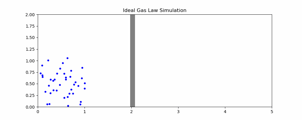
In the simulation, when particles hit the moving wall, it is pushed back proportional to the x component of the particle's velocity. We can quantity the pressure as the frequency of collision and the speed of the particles hitting it. With the current parameters, width hovers around 2. How would changing the parameters affect the size of the container?

If the volume of the container is increased, it takes longer for particles to hit the moving wall, decreasing the pressure as the frequency of collisions is reduced even though particle speed is unaffected
If the temperature is increased, the particles will be moving faster on average. Since the amount by which the wall is pushed is proportional to the speed, this means an increase in volume
If the number of particles is increased, there will be more frequent collisions with the moving wall, increasing volume
If we increase the external pressure (the speed that the wall moves left when it isn't being hit), then the volume of the container will decrease.

Extensions of the Ideal Gas Law

Van der Waals Equation

The Van der Waals equation is a modification of the Ideal Gas Law that takes into account the finite size of molecules and the intermolecular forces between them. The equation is expressed as: $$\left(P+a(\frac{n}{V})^2\right)(V-nb)=nRT$$ a and b are Van der Waals constants specific to the specie that takes into account intermolecular forces and size of the molecule, respectively.

Virial Equation

The Virial Equation is a power series extension. $$\frac{PV}{RT}=A+\frac{B}{V}+\frac{C}{V^2}+\dots$$ where A,B,C,$\dots$ are molecule-specific coefficients that depend on temperature

PV Diagrams

One useful tool for understanding thermodynamic processes is Pressure-Volume Diagrams. This plots the path that a system takes, plotted by its pressure and volume. There are four main types of processes that we will consider:

Isothermal: constant temperature process
Isobaric: constant pressure process
Isochoric: constant volume process
Adiabatic: No heat exchange

Isothermal Process

An isothermal process has constant temperature over the duration of the process. Since pressure and volume are inversely proportional with everything else being held constant, the curve behaves like y=1/x. In our monoatomic ideal gas, the energy of the system stays constant as N and T are unchanging. By the first law, this means that the heat transfer must be equal to the negative of the work. If the system expands and does x Joules of work, then x Joules of heat must flow into the system from the surroundings. Isotherm curves give the possible states for a given temperature and mole.

The effect that temperature has on the set of states can be observed in the following figure:

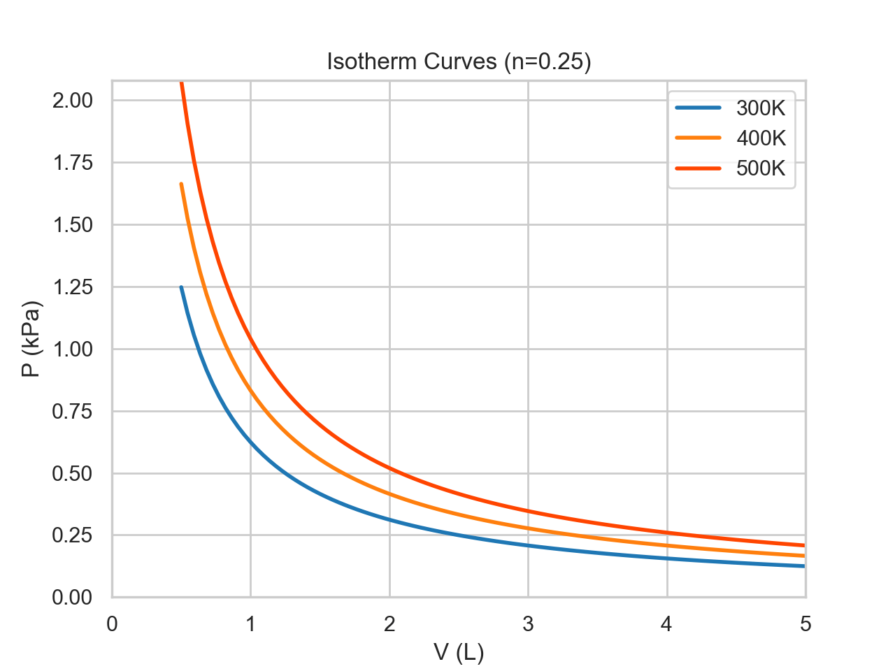
def ideal_gas(V,T,n):
    # PV=nRT
    R = 8.314
    return n*R*T/V/1000 # for kPa

x_values = np.linspace(.5,5,100)
n = 0.25
T1 = 300
T2 = 400
T3 = 500


fig = plt.figure()

plt.ylim([0,ideal_gas(x_values[0],T3,n)])
plt.xlim([0,5])

plt.plot(x_values,
            [ideal_gas(x,T1,n) for x in x_values],linewidth=2,color='tab:blue')
plt.plot(x_values,
            [ideal_gas(x,T2,n) for x in x_values],linewidth=2,color='gold')
plt.plot(x_values,
            [ideal_gas(x,T3,n) for x in x_values],linewidth=2,color='orangered')


plt.ylabel('P (kPa)')
plt.legend(['300K','400K','500K'])

plt.title("Isotherm Curves (n=0.25)")
plt.xlabel('V (L)')

plt.show()

Isobaric Process

In an isobaric process, the pressure remains constant throughout. Temperature and volume will both change proportional to one another. In an isobaric process, the work is easy to calculate as P is constant, so the work is just $P\Delta V$. The temperature and energy will increase if the volume increases and the opposite happens if the volume decreases.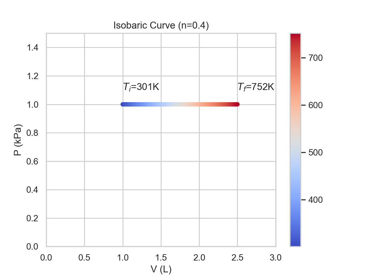

def ideal_gas_temp(V,p,n):
    # PV=nRT
    R = 8.314
    return round(V*p/n/R*1000) # for kPa

x_values = np.linspace(1,2.5,100)
n = 0.4

fig = plt.figure()

plt.ylim([0,1.5])
plt.xlim([0,3])

plt.scatter(x_values,
            [1 for i in x_values],
            linewidth=1,
            cmap='coolwarm',
            c=[ideal_gas_temp(i,1,n) for i in x_values])

plt.ylabel('P (kPa)')

plt.title(f"Isobaric Curve (n={n})")
plt.xlabel('V (L)')
plt.annotate(f'$T_i$={ideal_gas_temp(x_values[0],1,n)}K',
                (x_values[0],1.1))
plt.annotate(f'$T_f$={ideal_gas_temp(x_values[-1],1,n)}K',
                (x_values[-1],1.1))
plt.colorbar()
plt.show()

Isochoric (Isovolumetric) Process

In an isochoric process, the volume remains constant throughout. Temperature and pressure will both change proportional to one another. Since there is no change in volume, there is no work being done. The change in temperature and energy shares the same sign as the change in pressure. Since there is no work being done, the change in energy is solely due to heat exchange with the surrounding.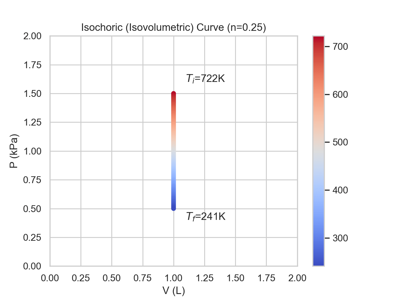

def ideal_gas_temp(V,p,n):
    # PV=nRT
    R = 8.314
    return round(V*p/n/R*1000) # for kPa

x_values = np.ones(100)
y_values = np.linspace(1.5,0.5,100)
n = 0.25

fig = plt.figure()

plt.ylim([0,2])
plt.xlim([0,2])

plt.scatter(x_values,
            y_values,
            linewidth=.5,
            cmap='coolwarm',
            c=[ideal_gas_temp(x_values[i],
                                y_values[i],n) for i in range(len(x_values))])

plt.ylabel('P (kPa)')

plt.title(f"Isochoric (Isovolumetric) Curve (n={n})")
plt.xlabel('V (L)')
plt.annotate(f'$T_i$={ideal_gas_temp(x_values[0],y_values[0],n)}K',
                (x_values[0]+0.1,y_values[0]+0.1))
plt.annotate(f'$T_f$={ideal_gas_temp(x_values[-1],y_values[-1],n)}K',
                (x_values[-1]+0.1,y_values[-1]-0.1))
plt.colorbar()
plt.show()

Adiabatic Process

In an adiabatic process, the PV curve looks similar to an isotherm, except it is steeper. An adiabatic expansion will decrease the temperature, doing work to expand the container. An adiabatic compression will increase the temperature. No heat is exchanged during this process; thus, the change in energy is equivalent to the work.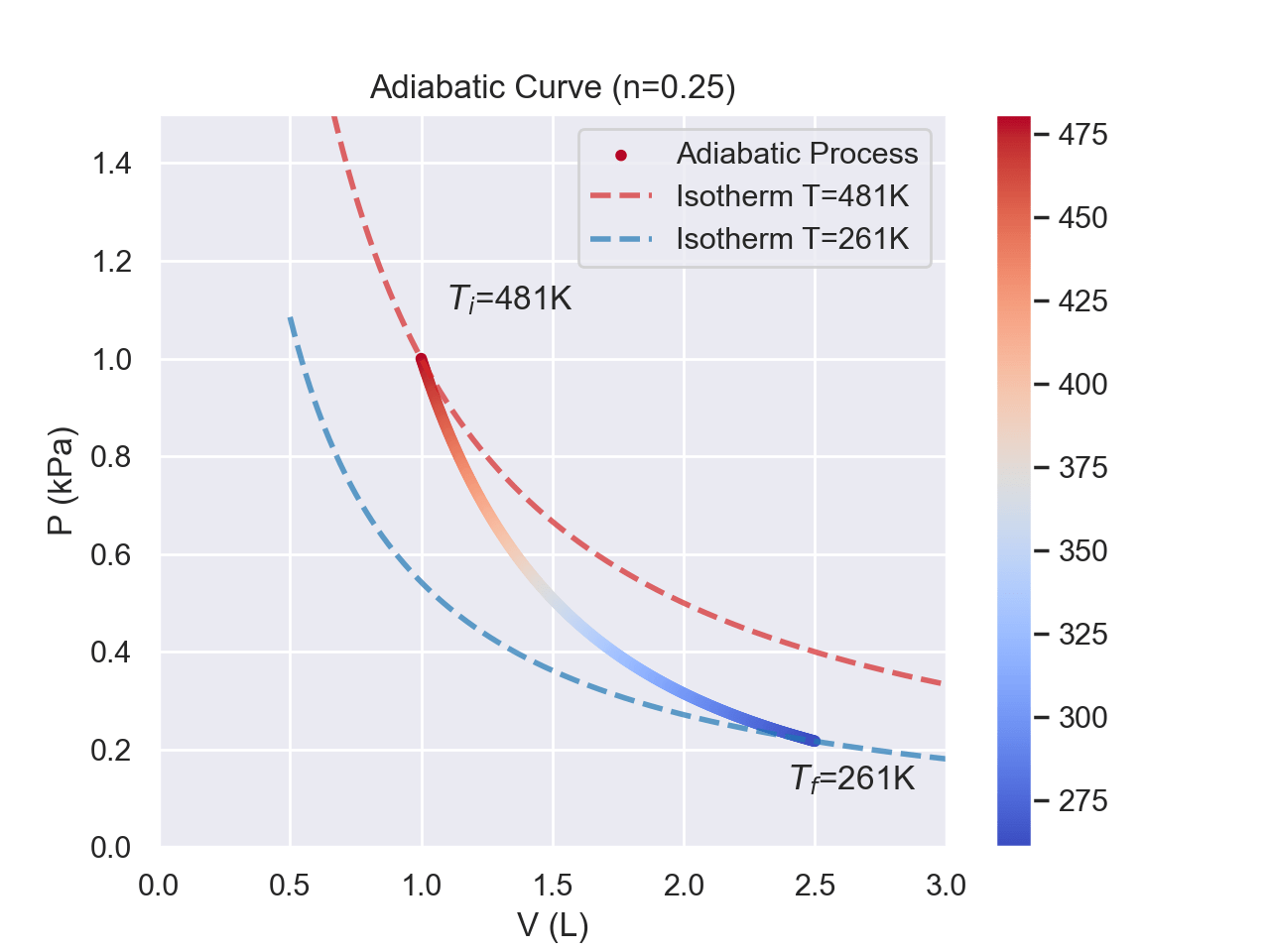

def ideal_gas_temp(V,p,n):
    # PV=nRT
    R = 8.314
    return round(V*p/n/R*1000) # for kPa

def ideal_gas(V,T,n):
    # PV=nRT
    R = 8.314
    return n*R*T/V/1000 # for kPa

def adiabatic_line(V):
    return 1/(V**(5/3))

x_values = np.linspace(1,2.5,100)
y_values = [adiabatic_line(i) for i in x_values]
n = 0.25
T1 = ideal_gas_temp(x_values[0],y_values[0],n)
T2 = ideal_gas_temp(x_values[-1],y_values[-1],n)
print(T1)
fig = plt.figure()

plt.ylim([0,2])
plt.xlim([0,4])

plt.scatter(x_values,
            y_values,
            linewidth=.5,
            cmap='coolwarm',
            c=[ideal_gas_temp(x_values[i],
                                y_values[i],n) for i in range(len(x_values))])
plt.plot(x_values,
            [ideal_gas(x,T1,n) for x in x_values],linewidth=2,color='tab:blue')
plt.plot(x_values,
            [ideal_gas(x,T2,n) for x in x_values],linewidth=2,color='gold')

plt.ylabel('P (kPa)')

plt.title(f"Adiabatic Curve (n={n})")
plt.xlabel('V (L)')
plt.annotate(f'$T_i$={ideal_gas_temp(x_values[0],y_values[0],n)}K',
                (x_values[0]+0.1,y_values[0]+0.1))
plt.annotate(f'$T_f$={ideal_gas_temp(x_values[-1],y_values[-1],n)}K',
                (x_values[-1]+0.1,y_values[-1]-0.1))
plt.legend(['Adiabatic Process','Isotherm T=481K','Isotherm T=261K'])
plt.colorbar()
plt.show()

Adiabatic Free Expansion

In adiabatic free expansion, the gas is expanding against a vacuum. Since there is no exterior pressure that it must fight while the container expands, the work is 0 as well. This also means no change in internal energy. The process is irreversible, however, and has a positive entropy change despite the lack of heat. This is an example of the Clausius Inequality which we will see next chapter.

Work: Area under the Curve

Because work and heat are inexact differentials, two paths that have the same start and end states will not necessarily have the same heat or work. This is a benefit of using PV curves, as the work can easily be calculated from finding the area under the curve. The figure below is an example of two paths that have different amount of work extracted. When going from left to right, the area under the curve is the work done by the system. When going from right to left, the area udner the curve is the work done to the system.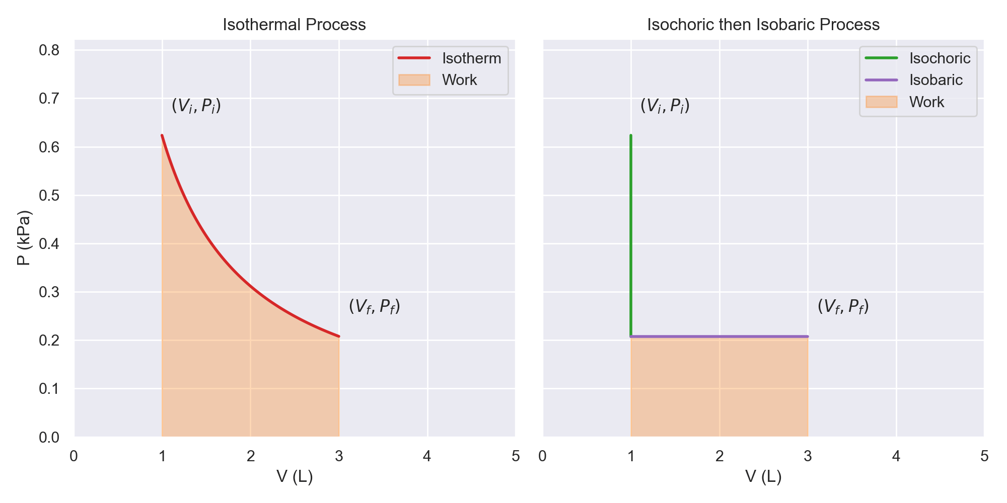

Isothermal Isochoric Isobaric Processes — Efficient versus Inefficient Work Paths

def ideal_gas(V,T,n):
    # PV=nRT
    R = 8.314
    return n*R*T/V/1000 # for kPa
x_values = np.linspace(1,3,100)
n = 0.25
T = 300
target_p = ideal_gas(x_values[-1],T,n)

fig, axes = plt.subplots(1,2,
                         sharey=True,
                         figsize=(10,5))

axes[0].set_ylim([0,ideal_gas(x_values[0],T,n)])
axes[0].set_xlim([0,5])

axes[0].plot(x_values,
            [ideal_gas(x,T,n) for x in x_values],
             linewidth=2,color='tab:red')

axes[0].fill_between(x_values,
                     [ideal_gas(x,T,n) for x in x_values],
                     alpha=0.3,color='tab:orange')
axes[0].set_ylabel('P (kPa)')
axes[0].legend(['Isotherm','Work'])

axes[0].set_title("Isothermal Process")
axes[0].set_xlabel('V (L)')

# least efficient

axes[1].set_ylim([0,ideal_gas(x_values[0],T,n)])
axes[1].set_xlim([0,5])

axes[1].plot([x_values[0],x_values[0]],
            [ideal_gas(x_values[0],T,n),
             ideal_gas(x_values[-1],T,n)],
             linewidth=2,
             color='tab:green',
             label='Isochoric')
plt.plot([x_values[0],x_values[-1]],
            [ideal_gas(x_values[-1],T,n),
             ideal_gas(x_values[-1],T,n)]
         ,linewidth=2,
         color='tab:purple',
         label='Isobaric')

plt.fill_between(x_values,
                 [ideal_gas(x_values[-1],T,n) for x in x_values],
                 alpha=0.3,
                 color='tab:orange',
                 label='Work')

axes[1].set_title("Isochoric then Isobaric Process")
plt.legend()


plt.xlabel('V (L)')
plt.tight_layout()
plt.show()

However, it is important to note that not all paths are possible. The isothermal process is the most efficient going both ways.

The work done by the system in an isothermal process is the maximum work that can extracted going from the initial state to the final state. Paths going from left to right must go below this curve.
The work done to the system in an isothermal process is the minimum work that can inputted to go from the initial state to the final state. Paths going from right to left must go above this curve.

Thermodynamic Cycles

Introduction

Thermodynamic cycles are sequences of processes that start and end in the same state, typically involving the transfer of heat and work. These cycles are fundamental in understanding how energy is converted and transferred in thermodynamic system

Carnot Cycle

The Carnot cycle is a theoretical cycle that represents the maximum possible efficiency a heat engine can achieve. It consists of two isothermal (constant temperature) and two adiabatic (no heat transfer) processes: It has the following steps:

Isothermal Expansion

The working substance (e.g., an ideal gas) undergoes an isothermal expansion at a high temperature $T_H$, absorbing heat $Q_H$ from the hot reservoir.

Adiabatic Expansion

The system expands adiabatically, with no heat exchange with the surroundings. The temperature of the system decreases during this process.

Isothermal Compression

The system is in contact with a cold resevoir at temperature $T_C$ and undergoes isothermal compression, expelling heat $Q_C$ to the cold resevoir.

Adiabatic Compression

The system is compressed adiabatically, with no heat exchange. The temperature of the system increases during this process.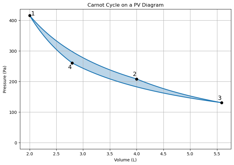

import matplotlib.pyplot as plt
import numpy as np

# Define parameters
R = 8.314  # Ideal gas constant
n = .25  # number of moles
T_H = 400  # High temperature
T_C = 350  # Low temperature
V_1 = 2    # Initial volume
V_2 = 4    # Final volume of isothermal expansion
gamma = 1.4  # heat capacity ratio
# Using the relationship PV^gamma = constant to find V_3
V_3 = V_2 * (T_H/T_C)**(1/(gamma-1))
V_4 = V_1 * (T_H/T_C)**(1/(gamma-1))


# Isothermal Expansion (1 to 2)
V_iso_exp = np.linspace(V_1, V_2, 100)
P_iso_exp = n * R * T_H / V_iso_exp

# Adiabatic Expansion (2 to 3)

V_adiab_exp = np.linspace(V_2, V_3, 100)
P_adiab_exp = P_iso_exp[-1] * (V_2**gamma) / (V_adiab_exp**gamma)

# Isothermal Compression (3 to 4)

V_iso_comp = np.linspace(V_3, V_4, 100)
P_iso_comp = n * R * T_C / V_iso_comp

# Adiabatic Compression (4 to 1)
V_adiab_comp = np.linspace(V_4, V_1, 100)
# Correcting the equation for adiabatic compression
P_adiab_comp = P_iso_exp[0] * (V_1**gamma) / (V_adiab_comp**gamma)

# Plotting the Carnot cycle
plt.figure(figsize=(9, 6))
plt.plot(np.concatenate((V_iso_exp, V_adiab_exp, V_iso_comp, V_adiab_comp)),
            np.concatenate((P_iso_exp, P_adiab_exp, P_iso_comp, P_adiab_comp)),linewidth=2)

plt.fill_between(np.concatenate((V_iso_exp, V_adiab_exp, V_iso_comp, V_adiab_comp)),
            np.concatenate((P_iso_exp, P_adiab_exp, P_iso_comp, P_adiab_comp)),alpha=0.3)

plt.scatter([V_iso_exp[0],V_adiab_exp[0],V_iso_comp[0],V_adiab_comp[0]],
            [P_iso_exp[0],P_adiab_exp[0],P_iso_comp[0],P_adiab_comp[0]],color='black',zorder=10)

# Annotating the plot
plt.text(V_1+.1, n * R * T_H / V_1, '1', fontsize=14, ha='right')
plt.text(V_2, n * R * T_H / V_2+10, '2', fontsize=14, ha='right')
plt.text(V_3, n * R * T_C / V_3+10, '3', fontsize=14, ha='right')
plt.text(V_4, n * R * T_C / V_4-20, '4', fontsize=14, ha='right')

plt.title('Carnot Cycle on a PV Diagram')
plt.xlabel('Volume (L)')
plt.ylabel('Pressure (Pa)')
plt.grid(True)
plt.show()

Heat Capacity

Heat capacity is the amount of heat required to raise the temperature of a system by 1 degree. There are two main types of heat capacities that we will consider, constant volume and constant pressure. $$C=\frac{\partial Q}{\partial T}$$

Constant Volume

We saw earlier that at constant volume, the heat was equal to the energy change. Thus, at a constant volume, we get the relationship. $$C_v=(\frac{\partial E}{\partial T})_V$$

Constant Pressure

$$C_p=(\frac{\partial Q}{\partial T})_p$$ We saw earlier that the change in enthalpy is equal to heat at constant pressure. $$C_p=(\frac{\partial H}{\partial T})_p$$ The heat capacity at constant pressure is greater than that at constant volume. The relationship between the constant pressure and constant volume heat capacities is given by $$C_p=C_v+nR$$ But intuitively, why is the heat capacity greater? Well, in a constant pressure environment, some of the heat going into the system is going towards doing work. This extra consideration is what leads to the difference.

Common Chemistry Equations

Gibbs Free Energy

Gibbs free energy is a common quantity to work with in Chemistry instead of energy, as it takes into account entropy. The common way that Gibbs Free enrgy is introduced in general chemistry is through the equations: $$\Delta G^0 = \Delta H^0 - T\Delta S^0$$ We can relate the Gibbs Free Energy to the equilibrium constant: $$\Delta G^0 = -RT\ln(K_{eq})$$ What is the standard state? We define it as having all the chemical species being 1M in concentration (except water). Even though this may not be a realistic scenario, we need some reference point to capture the inherent nature of the reaction. We can then adjust that value to take into account the actual concentrations in order to give us the real change in Gibbs free energy, $\Delta G$. $$\Delta G = \Delta G^0 + RT\ln(Q)$$

Thermodynamics Exercises

How does the area under the curve on a PV diagram relate to the work done by or on the system?
Compare the work done in an isothermal versus an adiabatic expansion of an ideal gas.
Define the first law of thermodynamics.
Define state functions and provide three examples.
For an ideal gas undergoing isothermal expansion, discuss the changes in internal energy, work, and heat.
Using the concept of free energy, explain why certain endothermic reactions can still be spontaneous.