k_M = 4e-4
k_cat = 10
E_0 = 1e-12
S_array = np.geomspace(1e-5,1e-2,100)
v_array = k_cat*E_0*S_array/(k_M+S_array)
noise = np.random.normal(size=(100))*5e-14
v_array = v_array + noise
plt.figure(figsize=(14,8))
plt.scatter(S_array, v_array,s=5)
plt.plot(S_array,
[0.5*1e-11 for i in range(100)],
color='red',alpha=0.5)
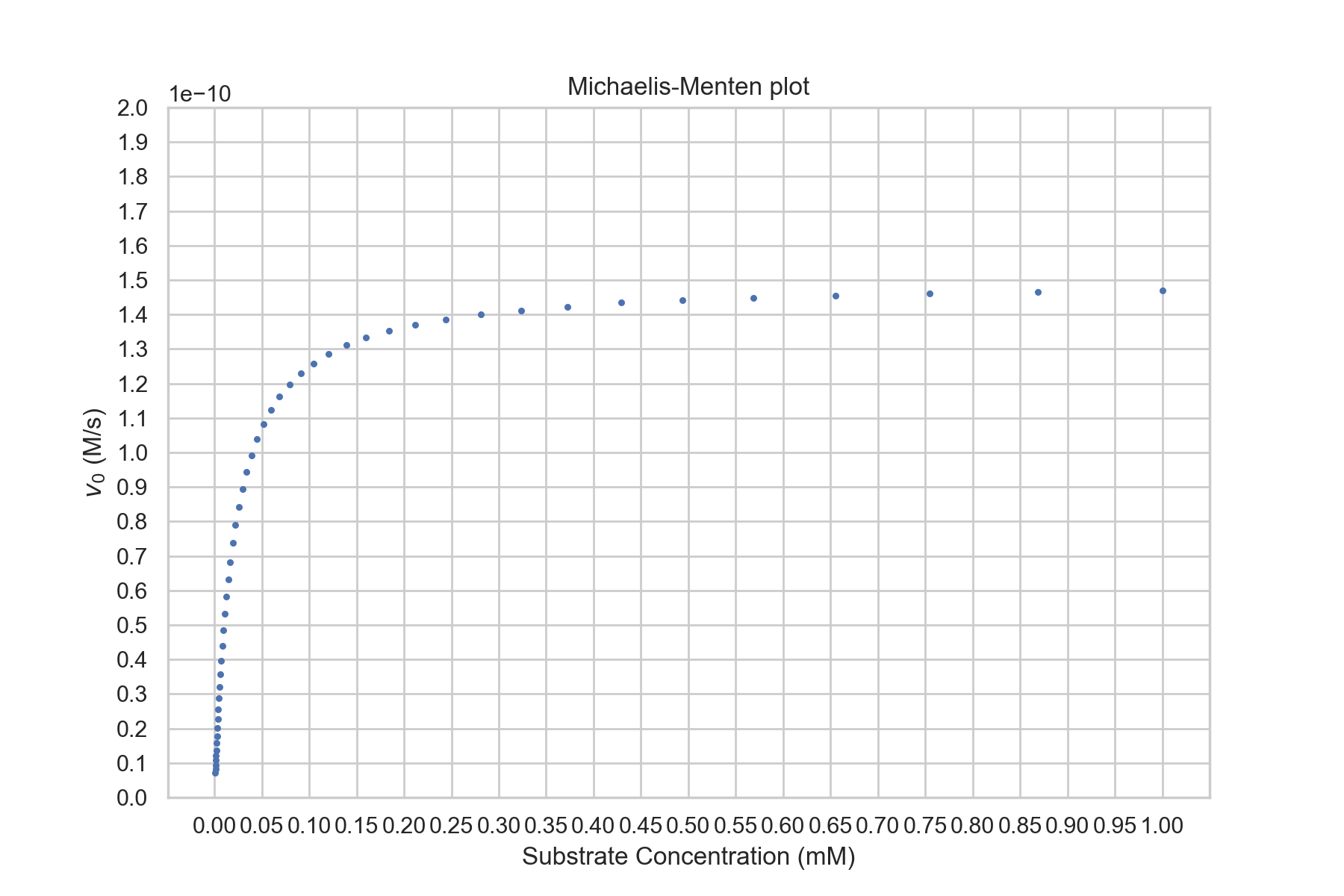
plt.title("Michaelis-Menten plot")
plt.xlabel("Substrate Concentration (M)")
plt.ylabel(f"$v_0$ (M/s)")
plt.xticks([i*5e-4 for i in range(0,21)])
plt.yticks([i*1e-12 for i in range(0,11)])
plt.show()
Michaelis-Menten Kinetics
Introduction
Michaelis-Menten kinetics is a fundamental concept in enzymology, describing the mathematical representation of enzyme-catalyzed reactions. It provides a framework for understanding how enzymes interact with substrates to form products and is crucial for interpreting experimental data related to enzyme reactions.Binding and Unbinding
Let us picture a an enzymatic reaction. We have a substrate, S, which binds to an Enzyme, E, resulting in a bound complex, \(E\cdot S\). After some amount of time, the substrate is transformed into product, P, and the enzyme unbinds. We will have the formation of the Enzyme-substrate complex be reversible, but consider the product formation to be irreversible. $$S+E\rightleftharpoons_{k_{-1}}^{k_1} E\cdot S \rightarrow^{k_{cat}} E+P$$Assumptions of Michaelis-Menten
Steady-State
The steady-state assumption posits that during the enzyme-substrate reaction, the concentration of the enzyme-substrate complex remains constant over time. $$\frac{d[E\cdot S]}{dt}=0$$Rapid Equilibrium
Enzyme-substrate binding and unbinding processes reach equilibrium much faster than the catalytic step of converting substrate to product.Single Substrate Reaction
The mechanism involves a single substrate molecule binding to the enzyme.Substrate and Enzyme Concentration
The assumption that the enzyme concentration is much lower than the substrate concentration, which simplifies the mathematical treatment of the kinetics.No Reverse Reaction
The assumption that the product does not rebind significantly to the enzyme to form the enzyme-substrate complex againDerivation of Kinetics Equation
There is a fixed amount of enzyme - either the enzyme is bound or unbound. Let us call the total amount of Enzyme, \(E_0\) $$E_0=[E]+[E\cdot S]$$ We can write general, complex rate laws by looking at the flux into and out of each state $$\frac{d[X]}{dt}=\sum R_i-\sum R_{j}$$ where R_i is the rate for a reaction step that produces X and R_j is the rate for a reaction step that depletes X. $$\frac{d[S]}{dt}=k_{-1}[E\cdot S]-k_1[E][S]$$ $$\frac{d[E]}{dt}=k_{-1}[E\cdot S]+k_{cat}[E\cdot S]-k_{1}[E][S]$$ $$=(k_{-1}+k_{cat})[E\cdot S]-k_1[E][S]$$ $$\frac{d[P]}{dt}=k_{cat}[E\cdot S]$$ $$\frac{d[E\cdot S]}{dt}=k_1[E][S]-k_{-1}[E\cdot S]-k_{cat}[E\cdot S]$$ A "steady-state approximation" is then made; that is, we treat the intermediate complex's concentration as a constant. $$\text{Let }\frac{d[E\cdot S]}{dt}=0$$ Using our above equations, we can then get $$k_{1}[E][S]=(k_{-1}+k_{cat})[E\cdot S]$$ Since we are ultimately interested in the rate of product formation, we should look to that equation for a possible next step. $$\frac{d[P]}{dt}=k_{cat}[E\cdot S]$$ Since we see that there is \([E\cdot S]\), we should manipulate the previous equation to find \([E\cdot S]\) in terms of [E] and [S], especially since we do not directly know the concentration of the enzyme-substrate complex. We know how much substrate and enzyme there are initially. We also do not necessarily know how much unbound enzyme there is either as that would also require knowledge of how much bound enzyme there was. So let's try to reduce it from 2 unknowns to 1 unknown. Another assumption that we will make is that \([S]\gg E_0\) since technically \(S_0=[S]+[E\cdot S]\), but we shall say \([S]+[E\cdot S]\approx [S]\). By using our total enzyme equation above, we can get $$k_{1}(E_0-[E\cdot S])[S]=(k_{-1}+k_{cat})[E\cdot S]$$ Let's now algebraically manipulate the equation to isolate \(E\cdot S\).. $$k_{1}E_0[S]-k_{1}[E\cdot S][S]=(k_{-1}+k_{cat})[E\cdot S]$$ $$k_{1}E_0[S]=(k_{1}[S]+(k_{-1}+k_{cat}))[E\cdot S]$$ $$[E\cdot S]=\frac{k_1E_0[S]}{k_1[S]+(k_{-1}+k_{cat})}$$ For simplicity, we will divide the numerator and denominator of the right side by \(k_1\) $$[E\cdot S]=\frac{E_0[S]}{\frac{k_{-1}+k_2}{k_1}+[S]}$$ We can then plug \(E\cdot S\) in to the rate of product formation equation $$\frac{dP}{dt}=k_{cat}[E\cdot S]$$ $$=\frac{k_{cat}E_0[S]}{\frac{k_{-1}+k_2}{k_1}+[S]}$$ While this result may look unruly, it does tell us some nice properties. Let us define a constant \(k_M\) $$k_M\equiv\frac{k_{-1}+k_{cat}}{k_1}$$ $$\frac{dP}{dt}=\frac{k_{cat}E_0[S]}{k_M+[S]}$$ When the susbtrate concentration is equal to \(k_M\), the rate of production is at 50% of max rate. $$V_{max}\equiv k_{cat}E_0$$Experimental Determination
Determining the kinetic parameters of enzymatic reactions, such as the Michaelis constant (\(K_M\)) and the maximum velocity (\(V_{max}\)), is typically done through an experimental process that involves measuring reaction rates under varying substrate concentrations. $$v=\frac{V_{max}[S]}{k_M+[S]}$$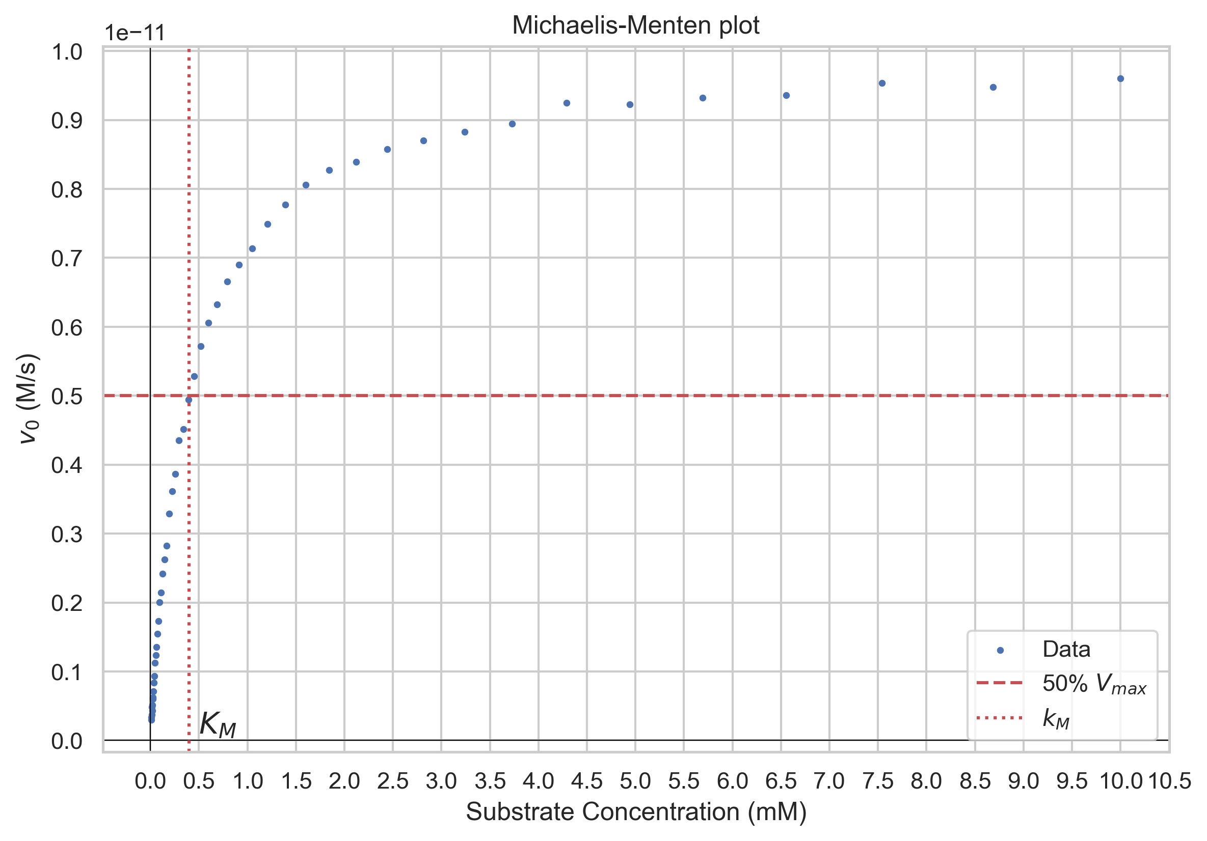
Linearization Methods for Michaelis-Menten Kinetics
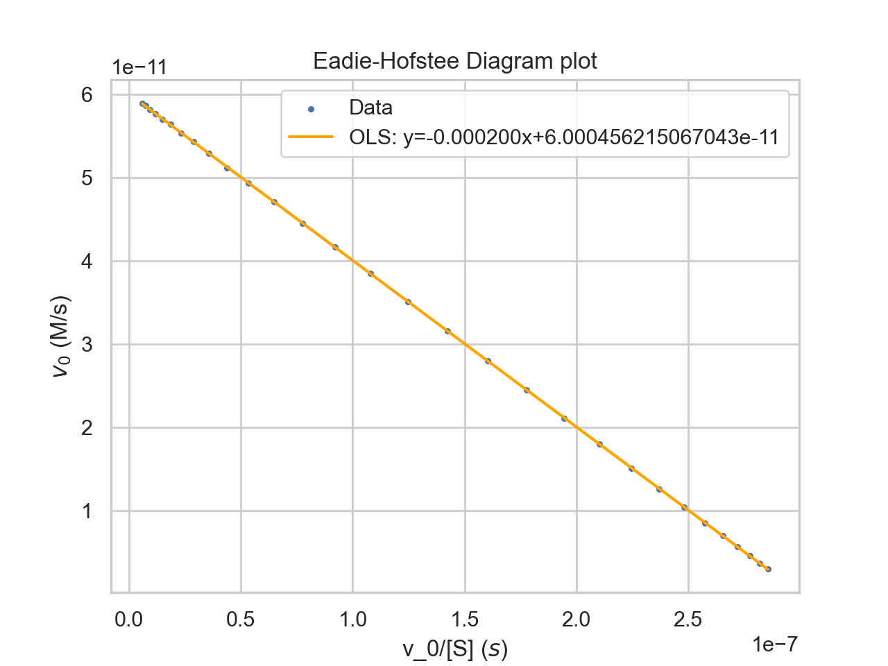
Since trying to estimate the half-max of a curve can be difficult, we might choose to linearize the data and use regression to find the best fit line and calculate the parameters from that. The three main linearization methods are Eadie-Hofstee, Hanes-Woolf, and Lineweaver-Burk.Eadie-Hofstee Plot
The Eadie-Hofstee diagram plots velocity against velocity divided by substrate concentration. The equation is given by $$v=V_{max}-K_M\frac{v}{[S]}$$ \(V_{max}\) is given by the y-intercept, and the Michaelis-Menten constant is given by the negative of the slope.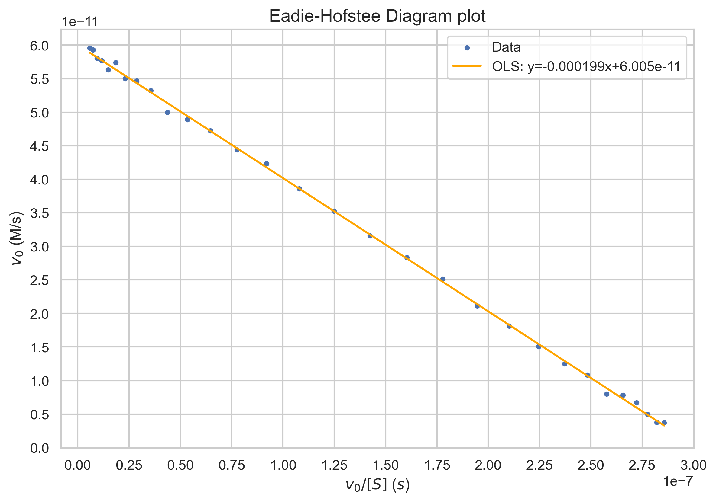
np.random.seed(0)
k_M = 4e-4
k_cat = 10
E_0 = 1e-12
S_array = np.geomspace(1e-5,1e-2,100)
v_array = k_cat*E_0*S_array/(k_M+S_array)
x_values = v_array/S_array

noise = np.random.normal(size=(100))*5e-14
v_array = v_array + noise
S_array_inverse = 1/S_array
v_array_inverse = 1/v_array
plt.figure(
    #figsize=(14,8)
)
plt.scatter(x_values, v_array,s=5)
model = sm.OLS(v_array,
                sm.add_constant(x_values))
results = model.fit()
plt.plot(x_values,
            results.predict(sm.add_constant(x_values)),
            color='orange')
plt.title("Eadie-Hofstee Diagram plot")
plt.xlabel("v_0/[S] ($s$)")
plt.ylabel(f"$v_0$ (M/s)")
plt.legend(['Data',
            f'OLS: y={results.params[1]:.6f}x+{results.params[0]}'])
plt.show()
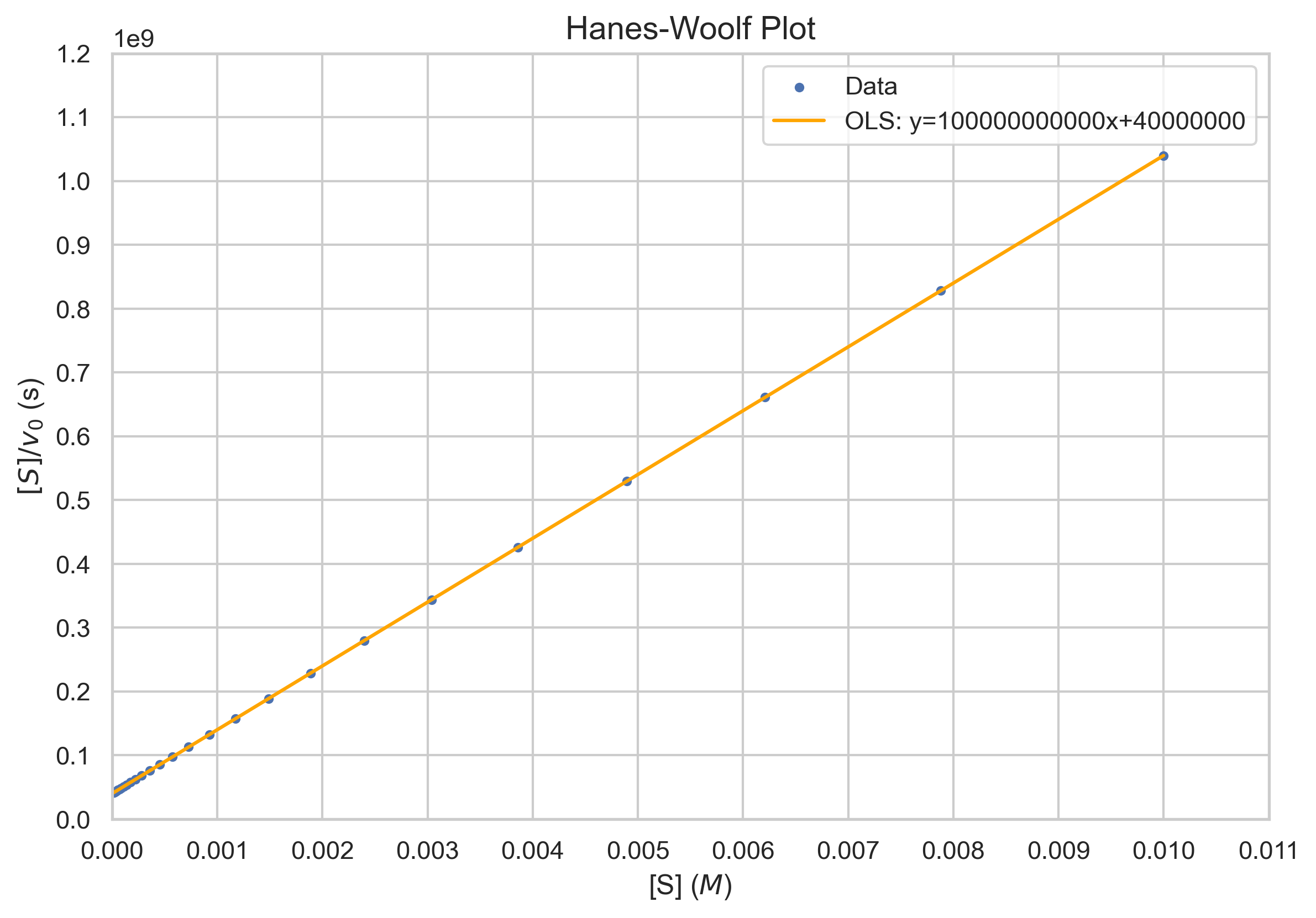
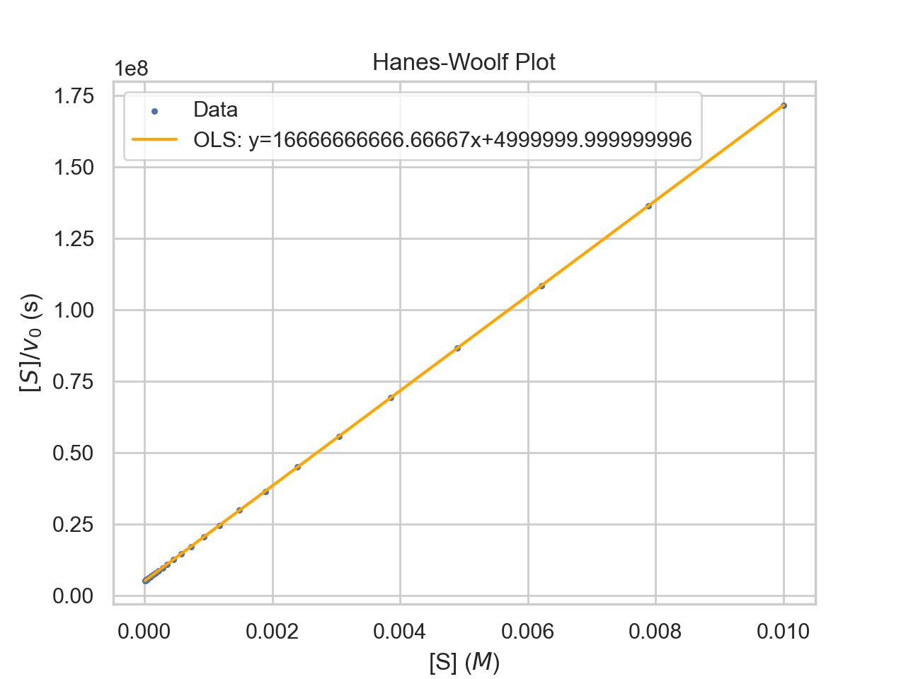
Hanes-Woolf Plot
The Hanes-Woolf plot is another linearization that plots [S]/v against [S]. The equation is given by $$\frac{[S]}{v}=\frac{1}{V_{max}}[S]+\frac{K_M}{V_{max}}$$ The slope is \(\frac{1}{V_{max}}\). The Michaelis-Menten constant is calculated from the y-intercept multiplied by \(V_{max}\).Considerations
Unlike the Lineweaver-Burk plot, the Hanes-Woolf plot tends to distribute errors more evenly, providing a more accurate linear representation of the data.However, it might be less intuitive for some researchers, especially when compared to the Lineweaver-Burk plot.
np.random.seed(0)
k_M = 4e-4
k_cat = 10
E_0 = 1e-12
S_array = np.geomspace(1e-5,1e-2,100)
v_array = k_cat*E_0*S_array/(k_M+S_array)
#x_values = v_array/S_array
y_values = S_array/v_array

noise = np.random.normal(size=(100))*5e-14
v_array = v_array + noise
S_array_inverse = 1/S_array
v_array_inverse = 1/v_array
plt.figure(
    #figsize=(14,8)
)
plt.scatter(S_array, y_values,s=5)
model = sm.OLS(y_values,
                sm.add_constant(S_array))
results = model.fit()
plt.plot(S_array,
            results.predict(sm.add_constant(S_array)),
            color='orange')
plt.title("Hanes-Woolf Plot")
plt.xlabel("[S] ($M$)")
plt.ylabel(f"$[S]/v_0$ (s)")
plt.legend(['Data',
            f'OLS: y={results.params[1]}x+{results.params[0]}'])
plt.show()
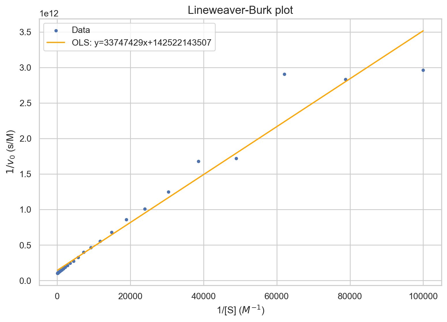
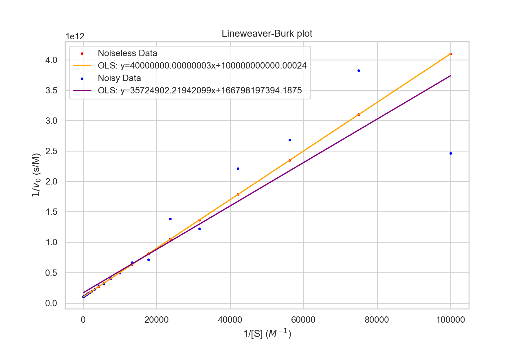
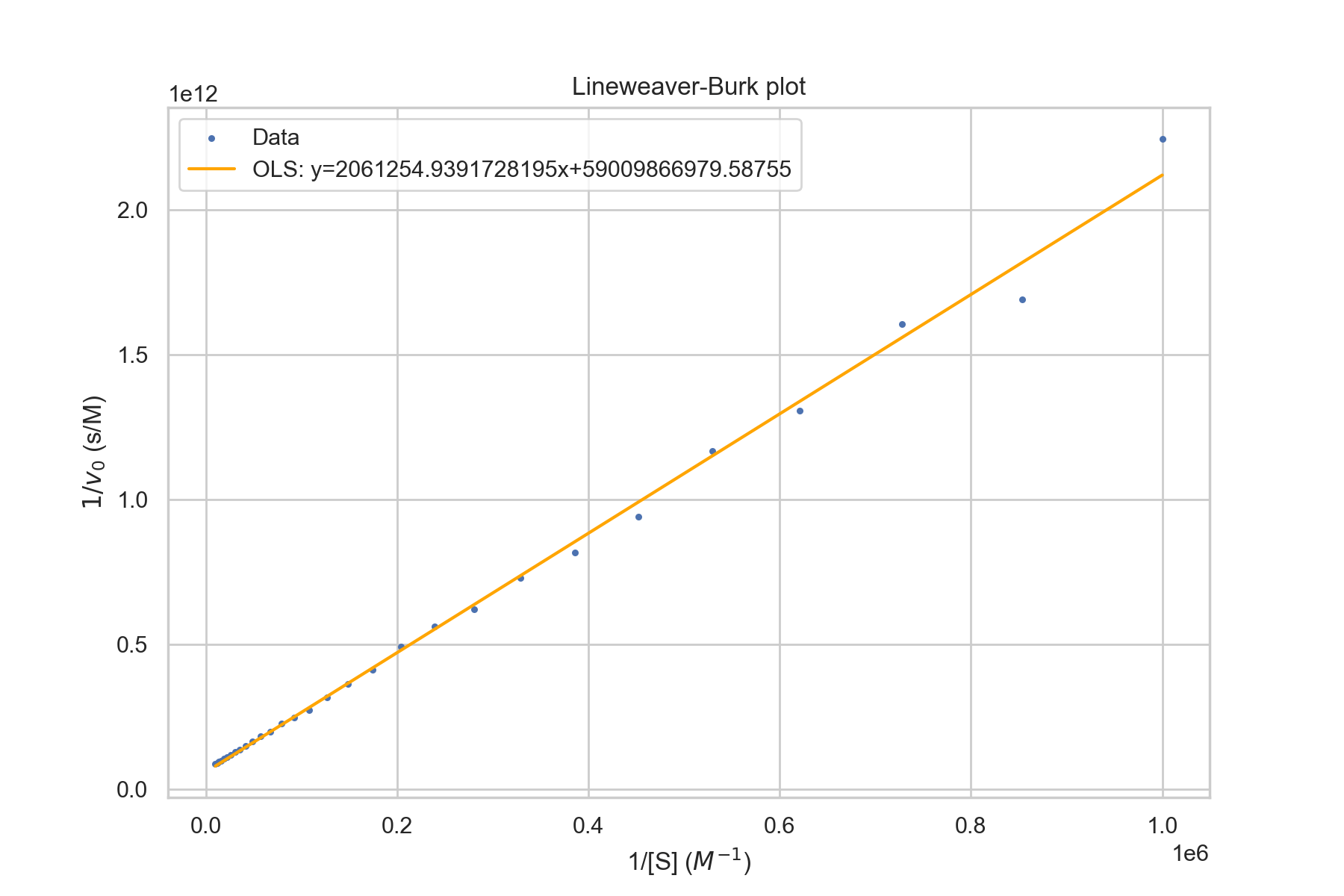
Lineweaver-Burk plot
One common method is Lineweaver-Burk plots, which are also called double-recipricol plots. As the name suggests, 1/[S] is plotted against 1/v. The y-intercept is 1/v_max. This is evident since as [S] goes to infinity, 1/[S] goes to 0. The slope is \(k_M/V_\text{max}\). The x-intercept is \(-1/k_M\).The Lineweaver-Burk equation is given by $$\frac{1}{v}=\frac{1}{V_{max}}+\frac{K_M}{V_{max}}\times\frac{1}{[S]}$$
k_M = 4e-4
k_cat = 10
E_0 = 1e-12
S_array = np.geomspace(1e-5,1e-2,100)
v_array = k_cat*E_0*S_array/(k_M+S_array)
noise = np.random.normal(size=(100))*5e-14
v_array = v_array + noise
S_array_inverse = 1/S_array
v_array_inverse = 1/v_array
plt.figure(figsize=(14,8))
plt.scatter(S_array_inverse, v_array_inverse,s=5)
model = sm.OLS(v_array_inverse,
                sm.add_constant(S_array_inverse))
results = model.fit()
plt.plot(S_array_inverse,
            results.predict(
                sm.add_constant(S_array_inverse)),
                color='orange')
plt.title("Lineweaver-Burk plot")
plt.xlabel("1/[S] ($M^{-1}$)")
plt.ylabel(f"$1/v_0$ (s/M)")
plt.legend(['Data',
            f'OLS: y={results.params[1]}x+{results.params[0]}'])
plt.show()
Noise and Estimations
One thing to note is the heteroskedasticity in the graph above. Ordinary Least Squares (OLS) is the best, unbiased linear model when the Gauss-Markov conditions are satisfied - one of which is homoskedasticity (variance of errors is constant over X). In practice, this can lead to bad estimates as the noisy values on the right can drastically affect the best-fit parameters. The following is a graph with Noiseless Michaelis-Menten data and the same data with noise \(\sim N(0,\sigma=1e-13)\). Note that the values are relatively similar.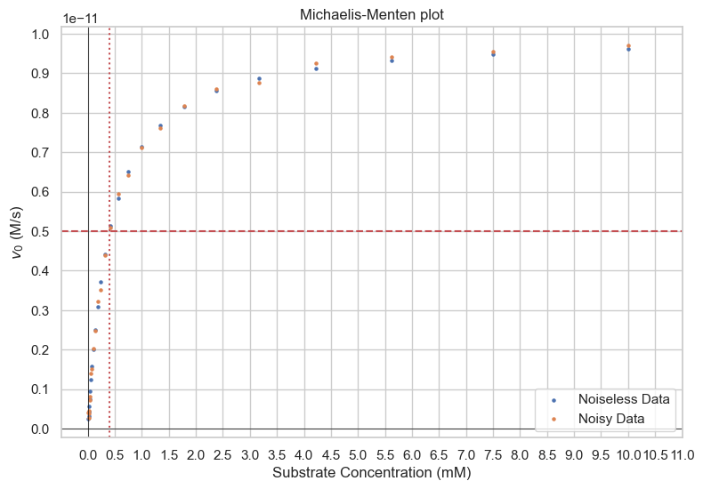
- Noiseless:
- \(v_{max}=\)1e-11 M/s
- \(k_M\)=4e-4 M
- With noise with std dev 1e-13:
- \(v_{max}=\)6e-12 M/s
- \(k_M=\)2.1e-4 M
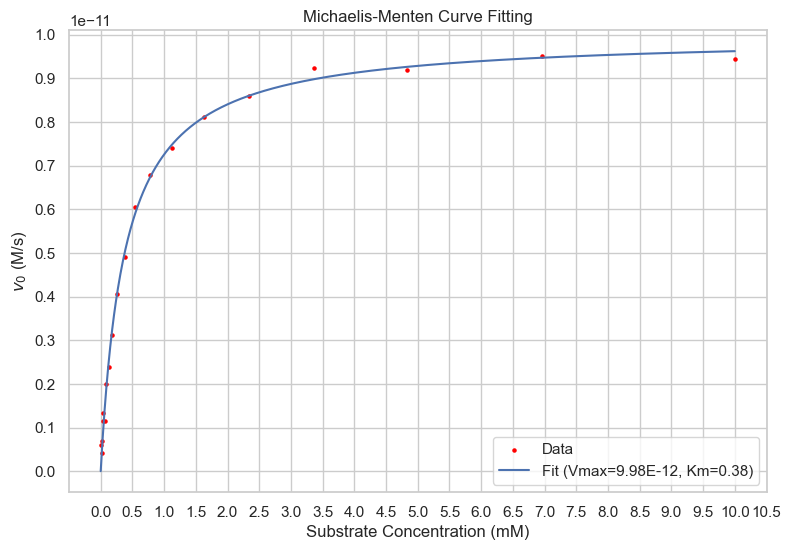
Curve Fitting
Non-linear curve fitting involves adjusting the parameters of a mathematical model to minimize the difference between the observed data and the model predictions, without linearizing the data or the model. Various software tools like GraphPad Prism, SigmaPlot, or specialized programs in R and Python, are available for performing non-linear curve fitting on enzyme kinetics data.Advantages
Unlike linearization methods, non-linear curve fitting does not distort the error structure of the data, providing more accurate estimates of parameters The parameters, \(V_{max}\) and \(K_m\) are directly estimated from the curve fitting, without the need for further transformation or interpretation.Drawbacks
Non-linear curve fitting often requires initial guesses for the parameters, and the results may be sensitive to these initial values.Non-linear curve fitting can be more complex and computationally intensive compared to linearization methods.
import numpy as np
from scipy.optimize import curve_fit
import matplotlib.pyplot as plt
import seaborn as sns

# Define the Michaelis-Menten function
def michaelis_menten(S, Vmax, Km):
    return (Vmax * S) / (Km + S)

# Sample data (substrate concentration and reaction velocity)
np.random.seed(0)
k_M = 4e-1
k_cat = 10
E_0 = 1e-12
sns.set_theme(style='whitegrid')
n = 20
S_array = np.geomspace(1e-2,1e1,n)
v_array = k_cat*E_0*S_array/(k_M+S_array)
noise = np.random.normal(size=(n))*2e-13
v_array = v_array + noise

# Perform the curve fitting
params, covariance = curve_fit(michaelis_menten, S_array, v_array, p0=[4, 1])

# Extract the fitted parameters
Vmax_fitted, Km_fitted = params

# Print the results
print(f'Fitted Vmax: {Vmax_fitted:}')
print(f'Fitted Km: {Km_fitted:.2f}')

# Generate fitted values for plotting
S_fitted = np.linspace(0, S_array.max(), 1000)
v_fitted = michaelis_menten(S_fitted, Vmax_fitted, Km_fitted)

# Plot the data and the fitted curve
plt.figure(figsize=(9,6))
plt.scatter(S_array, v_array, color='red', label='Data',s=5)
plt.plot(S_fitted, v_fitted, label=f'Fit (Vmax={Vmax_fitted*1e12:.2f}E-12, Km={Km_fitted:.2f})')
plt.title("Michaelis-Menten Curve Fitting")
plt.xlabel("Substrate Concentration (mM)")
plt.ylabel(f"$v_0$ (M/s)")
plt.xticks([i*5e-1 for i in range(0,22)])
plt.yticks([i*1e-12 for i in range(0,11)])
plt.legend()
plt.grid(True)
plt.show()
Enzyme Specificity
A common metric for enzyme efficiency is given by $$k_s=\frac{k_{cat}}{K_M}$$Inhibition
Enzyme inhibition is a crucial aspect of enzyme kinetics and pharmacology, affecting the rate of enzyme-catalyzed reactions. Understanding enzyme inhibition is vital in drug development, as many drugs act as enzyme inhibitors, modifying enzyme activity to achieve therapeutic effects. In this section, we explore the different types of enzyme inhibition: competitive, non-competitive, uncompetitive, and mixed inhibition.
By Athel cb - Own work, CC BY-SA 4.0, Link
Competitive Inhibition
We had previously just considered the scenario where the substrate had no competition for binding to the active site, but the equation can be extended easily to include the presence of another moelecule that can bind to the same active site as the substrate, but will not undergo the catalytic reaction. Let us assume the same dynamics, but with the addition of a side reaction: $$S+E\rightleftharpoons_{k_{-1}}^{k_1} E\cdot S \rightarrow^{k_{cat}} E+P$$ $$E+I\rightleftharpoons_{k_2}^{k_{-2}} E\cdot I$$ Since there is a new state can consume E to enter and product E when it leaves, this will change our equation for \(\frac{d[E]}{dt}\) as well as create new equations for \(\frac{d[E\cdot I]}{dt}\) and \(\frac{d[I]}{dt}\). We can denote the equilibrium constant for the association of the Enzyme-Inhibitor complex to be \(K_I\). $$K_I=\frac{k_{-2}}{k_2}$$ $$\frac{[E][I]}{[E\cdot I]}=K_I\sim\frac{[E]I_0}{[E\cdot I]}$$ $$E_0=[E]+[E\cdot S] +[E\cdot I]$$ $$[E]=E_0-[E\cdot S]-[E\cdot I]$$ $$[E]=E_0-[E\cdot S]-\frac{[E]I_0}{K_I}$$ $$[E](1+\frac{I_0}{K_I})=E_0-[E\cdot S]$$ $$[E]=\frac{E_0-[E\cdot S]}{1+\frac{I_0}{K_I}}$$ Let us define a constant \(\alpha\) such that $$\alpha\equiv 1+\frac{I_0}{K_I}$$ $$[E]=\frac{E_0-[E\cdot S]}{\alpha}$$ $$0=\frac{d[E\cdot S]}{dt}=k_1[E][S]-k_{cat}[E\cdot S]-k_{-1}[E\cdot S]$$ $$[E\cdot S](k_{cat}+k_{-1})=k_1[E][S]$$ $$[E\cdot S]=\frac{1}{K_M}[E][S]$$ $$\approx \frac{1}{k_M}[E]S_0$$ $$[E\cdot S]_{ss}=\frac{S_0}{k_M}\times\frac{E_0-[E\cdot S]_{ss}}{\alpha}$$ $$[E\cdot S]_{ss}(1+\frac{S_0}{k_M\alpha})=\frac{S_0E_0}{\alpha k_M}$$ $$[E\cdot S]_{ss}=\frac{\frac{S_0E_0}{k_M\alpha}}{1+\frac{S_0}{k_M\alpha}}$$ $$=\frac{E_0}{1+\frac{\alpha k_M}{S_0}}$$ Now finally plugging in the concentration into the product formation kinetic equation: $$v_0=k_{cat}[E\cdot S]_{ss}=\frac{k_{cat}E_0}{1+\frac{\alpha k_M}{S_0}}$$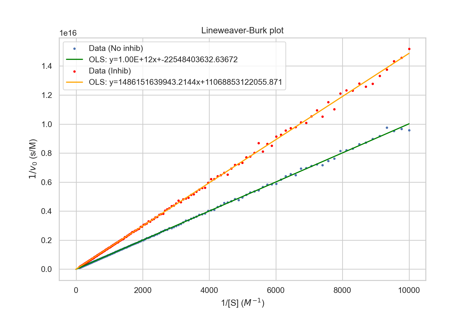
import decimal
np.random.seed(3)
k_M = 4e-4
k_cat = 10
E_0 = 1e-12
S_array = np.geomspace(1e-4,1e-2,200)
test_points = 1/np.array([-0.1,1e-4])

alpha = 1
v_array = k_cat*E_0/(1+k_cat*alpha/S_array)
noise = np.random.normal(size=(200))*.25e-17
v_array = v_array + noise
S_array_inverse = 1/S_array
v_array_inverse = 1/v_array
ax = plt.figure(figsize=(14,8))
plt.scatter(S_array_inverse,
            v_array_inverse,s=5)
model = sm.OLS(v_array_inverse,
                sm.add_constant(S_array_inverse))
results = model.fit()
plt.plot(test_points,
            results.predict(sm.add_constant(test_points)),
            color='green')

alpha = 1.5
v_array = k_cat*E_0/(1+k_cat*alpha/S_array)
noise = np.random.normal(size=(200))*.25e-17
v_array = v_array + noise
S_array_inverse = 1/S_array
v_array_inverse = 1/v_array
plt.scatter(S_array_inverse,
            v_array_inverse,s=5,
            color='red')
model2 = sm.OLS(v_array_inverse,
                sm.add_constant(S_array_inverse))
results2 = model2.fit()
plt.plot(test_points,
            results2.predict(
                sm.add_constant(test_points)),
                color='orange')


plt.title("Lineweaver-Burk plot")
plt.xlabel("1/[S] ($M^{-1}$)")
plt.ylabel(f"$1/v_0$ (s/M)")
plt.legend(['Data (No inhib)',
            f'OLS: y={results.params[1]:.2E}x+{results.params[0]}',
            'Data (Inhib)',
            f'OLS: y={results2.params[1]}x+{results2.params[0]}'])
plt.show()
- \(v_{\text{max}}\) stays the same
- \(k_M\) increases as more substrate is required to reach half max velocity
Uncompetitive Inhibition
Uncompetitive inhibition involves the following dynamics: $$S+E\rightleftharpoons_{k_{-1}}^{k_1} E\cdot S \rightarrow^{k_{cat}} E+P$$ $$E\cdot S+I\rightleftharpoons_{k_2}^{k_{-2}} E\cdot S\cdot I$$ With this form of inhibition, the inhibitor binds to the \(E\cdot S\) complex, not E, and prevents enzyme activity as well as substrate dissociation. In a Lineweaver-Burk plot, this would appear as a parallel shift downward. $$v_0=\frac{k_{cat}E_0[S]}{K_m+[S](1+[I]/K_{iu})}$$ where [I] is the concenntration of the uncompetitive inhibitor and \(K_{iu}\) is the uncompetitive inhibition constant. The following are the effects of uncompetitive inhibition:- \(v_{\text{max}}\) decreases
- \(k_M\) decreases
Non-competitive Inhibition
While similar in name to uncompetitive, non-competitive inhibition is distinct from it. Non-competitive inhibition does not involve the inhibitor binding to the active site, instead it binds to an "allosteric site." The inhibitor can bind to both E and \(E\cdot S\). Similarly, the substrate is able to bind and unbind to both E and \(E\cdot I\). $$S+E\rightleftharpoons_{k_{-1}}^{k_1} E\cdot S \rightarrow^{k_{cat}} E+P$$ $$E+I\rightleftharpoons_{k_2}^{k_{-2}} E\cdot I$$ $$E\cdot S+I\rightleftharpoons_{k_3}^{k_{-3}} E\cdot S\cdot I$$ $$E\cdot I + S \rightleftharpoons_{k_4}^{k_{-4}} E\cdot S\cdot I$$This has the effect of essentially reducing the amount of enzyme present, as if less had been added in the first place. The following are the effects of non-competitive inhibition: $$v=\frac{V_{max}}{(1+\frac{K_m}{[S]})(1+\frac{[I]}{K_i})}$$
- \(v_{\text{max}}\) decreases
- \(k_M\) is unaffected
Extensions
Briggs-Haldane
Introduction
The Briggs-Haldane model generalizes the Michaelis-Menten approach to enzyme kinetics by relaxing the assumption of a rapid equilibrium or a steady state between the enzyme-substrate complex and the product. This model is particularly useful for reactions where the dissociation of the enzyme-substrate complex into the product is comparable to its formation rate.Summary
This chapter aims to explore the principles and methodologies of Michaelis-Menten kinetics, along with the applications of Lineweaver-Burk, Hanes-Woolf, and Eadie-Hofstee plots. These techniques provide a foundational understanding of enzyme kinetics, allowing researchers to deduce critical parameters and investigate enzyme mechanisms and interactions.Understanding the different types of enzyme inhibition and their representation on various enzyme kinetics plots, including Lineweaver-Burk, Hanes-Woolf, and Eadie-Hofstee plots, is essential for deciphering the interaction between enzymes, substrates, and inhibitors. This knowledge is pivotal in biological research, allowing scientists to explore the regulatory mechanisms of enzymatic activities and develop therapeutic agents that modulate enzyme activity in specific pathological conditions.
Michaelis Menten Practice Exercises
- Define \(V_{max}\)
- If an enzyme has a Km of 5 mM and a Vmax of 10 µmol/min, what is the reaction velocity (V0) when the substrate concentration is:
- 5mM
- 10mM
- 1mM
- 20mM
- Given a graph of reaction velocity versus substrate concentration for an enzyme, determine:
- The approximate value of Km.
- The approximate value of Vmax.
- Compare and contrast competitive and non-competitive inhibitors in terms of their effect on Km and Vmax.
- Given an enzyme with a Vmax of 20 µmol/min and a Km of 4 mM, calculate the reaction velocity when the substrate concentration is 8 mM.
- How does enzyme concentration affect the value of Vmax?
- If an enzyme exhibits a Vmax of 100 µmol/min in the presence of a certain inhibitor and 150 µmol/min in its absence, is the inhibitor competitive or non-competitive?
- Sketch the Michaelis-Menten plot and the Lineweaver-Burk plot. Label the axes appropriately.
- What would be the reaction velocity if the substrate concentration was zero?
- Given an Eadie-Hofstee Diagram, determine:
- The approximate value of Km.
- The approximate value of Vmax.
- Given a Hanes-Woolf Plot, determine:
- The approximate value of Km.
- The approximate value of Vmax.
- Given a Lineweaver-Burk Plot, determine:
- The approximate value of Km.
- The approximate value of Vmax.
- What does a high Km value indicate about an enzyme's affinity for its substrate?
- Given the kinetic data for two different enzymes acting on the same substrate, how would you determine which enzyme is more efficient?
- Scenario: An inhibitor increases the Km of an enzyme from 5 mM to 20 mM but does not change the Vmax. Classify this inhibitor.
- True or False: A non-competitive inhibitor binds only to the enzyme-substrate complex.
- For a reaction following Michaelis-Menten kinetics, describe what is happening at the molecular level when the substrate concentration is much higher than the Km.
- Explain the basic principle behind non-linear curve fitting and how it differs from linearization methods.
- Describe the steps involved in performing non-linear curve fitting on Michaelis-Menten kinetics data.
- Discuss the advantages of using non-linear curve fitting for analyzing enzyme kinetics.
- What are some considerations and limitations when employing non-linear curve fitting in enzyme kinetics analysis?