import numpy as np
import matplotlib.pyplot as plt

def estimate_pi(num_samples):
    inside_circle = 0
    x_inside = []
    y_inside = []
    x_outside = []
    y_outside = []

    for _ in range(num_samples):
        x, y = np.random.uniform(0, 1, 2)  # Randomly sample point in square
        if x**2 + y**2 <= 1:  # Check if point is inside circle
            inside_circle += 1
            x_inside.append(x)
            y_inside.append(y)
        else:
            x_outside.append(x)
            y_outside.append(y)

    return (4.0 * inside_circle) / num_samples, x_inside, y_inside, x_outside, y_outside

num_samples = 10000
pi_estimate, x_inside, y_inside, x_outside, y_outside = estimate_pi(num_samples)

# Plotting
plt.figure(figsize=(8,8))
plt.scatter(x_inside, y_inside, color='blue', s=1)
plt.scatter(x_outside, y_outside, color='red', s=1)
plt.title(f"Estimation of Pi using {num_samples} samples: {pi_estimate}")
plt.xlabel('x')
plt.ylabel('y')
plt.grid(True)
plt.gca().set_aspect('equal', adjustable='box')
plt.show()
Monte Carlo Simulations
Introduction to Monte Carlo
The Monte Carlo method is a broad class of computational algorithms that rely on repeated random sampling to obtain numerical results. The basic concept is to use simulations with randomness to obtain results that may be unfeasible to obtain analytically or observationally.Basics of Monte Carlo
Outline of Monte Carlo Steps
- Defining a domain of possible inputs.
- Generating inputs randomly from a probability distribution over the domain.
- Performing a deterministic computation on the inputs.
- Aggregating the results
Defining A Domain of Possible Inputs
Some questions to ask:- What variables will be randomly generated?
- How often will they be generated per trial?
Generating Inputs
Appropriate distribution
What distribution will each variable be sampled from? Some common distributions for a given task:- Normal distribution: symmetric deviation from a value, with high probability of being around mean
- Log-Normal distribution: Relative changes are normally distributed
- Uniform distribution: Comparing versus probability threshold
- Beta: Randomly generating percentages
- Exponential distribution: Memory-less waiting for an event
- Poisson: Number of occurences when events are independent
- Half-normal distribution: Non-negative values with low kurtosis
- Bernoulli: binary outcome
- Binomial: repeated binary outcomes
How to Sample
For the common distributions, the sampling can be done by many libraries. For more complicated distributions, there are techniques such as inverse transform sampling.Sampling Techniques
There are a number of sampling techniques that can be used to reduce variance of the estimator.- Antithetic variates
- Control variates
- Importance sampling
Deterministic Computation
Aggregating Results
The Monte Carlo estimator has a standard deviation that scales with the inverse sequare root of n.Basic Example
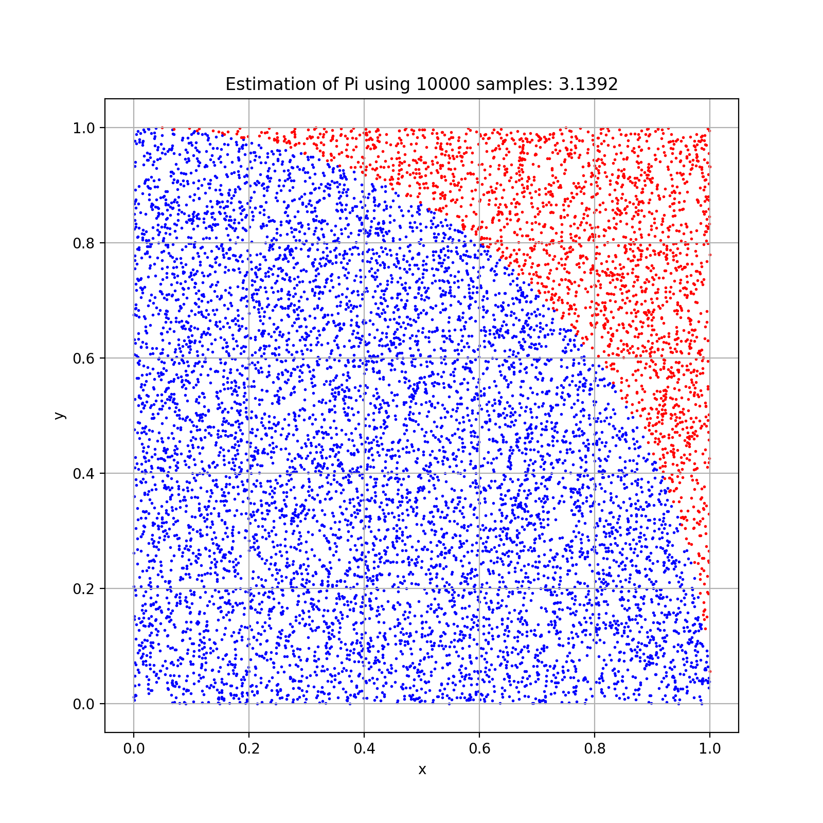
Monte Carlo is commonly introduced with estimating Pi, and we shall be no exception. If we wished to calculate pi or determine the area of a circle, we can randomly generate points on the set \([-r,r]\times [-r,r]\). The area of the circle would then be the percentage of points in the set \(\{x,y : x^2+y^2\leq r^2\}\) multiplied by the total area of the sample set, \((2r)^2=4r^2\). By symmetry, we can restrict the sampling to just one quadrant and the ratio of points within the circle to the total area will be the same. Since \(A_{c}=\pi r^2\), we can determine pi by the relationship $$\frac{A_c}{A_s}=\frac{\pi r^2}{4 r^2}=\frac{\pi}{4}$$ Thus pi is 4 times the fraction of points inside the circle (or quartercircle or semicircle),.
import numpy as np
import matplotlib.pyplot as plt

def estimate_pi(num_samples):
    inside_circle = 0
    x_inside = []
    y_inside = []
    x_outside = []
    y_outside = []

    for _ in range(num_samples):
        x, y = np.random.uniform(0, 1, 2)  # Randomly sample point in square
        if x**2 + y**2 <= 1:  # Check if point is inside circle
            inside_circle += 1
            x_inside.append(x)
            y_inside.append(y)
        else:
            x_outside.append(x)
            y_outside.append(y)

    return (4.0 * inside_circle) / num_samples, x_inside, y_inside, x_outside, y_outside

num_samples = 10000
pi_estimate, x_inside, y_inside, x_outside, y_outside = estimate_pi(num_samples)

# Plotting
plt.figure(figsize=(8,8))
plt.scatter(x_inside, y_inside, color='blue', s=1)
plt.scatter(x_outside, y_outside, color='red', s=1)
plt.title(f"Estimation of Pi using {num_samples} samples: {pi_estimate}")
plt.xlabel('x')
plt.ylabel('y')
plt.grid(True)
plt.gca().set_aspect('equal', adjustable='box')
plt.show()
Error in Monte Carlo
Sources of Error
Sampling Error
Arises due to the finite number of samples used in the simulation. As the number of samples increases, the sampling error decreases, but at the cost of computational resources.Model Error
Occurs when the model used in the simulation does not perfectly represent the real system being studied. This type of error is inherent to the model itself and cannot be reduced by increasing the number of samples.Estimation of Error
The standard error (SE) gives an estimate of the sampling error in the MC estimate. It is given by the formula: $$SE=\frac{s}{\sqrt{n}}$$ where s is the sample standard deviation and n is the number of samples.Biology Applications of Monte Carlo
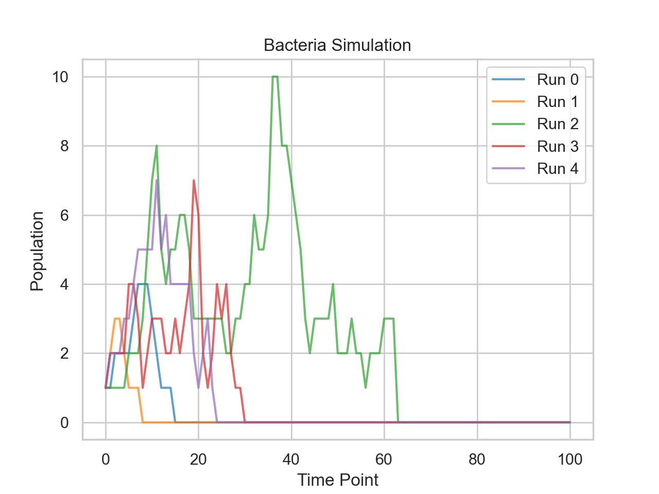
A classic example is modeling bacteria population.We can start with 1 bacterium. At each time point, it has a 25% chance to split into 2, a 25% chance to die, and 50% chance to do nothing. Using probability, you could get a closed form answer, but we can also model this easily. We can run many simulations and take an average to see what the expected number of bacteria are at a given time. One advantage is that we can easily change parameters and get results without having to do much work.
import numpy as np
sns.set_theme(style='whitegrid')
np.random.seed(1)
def simulate_bacteria_growth(steps=100, p_split=0.25, p_die=0.25):
    population = 1  # Start with a single bacteria
    populations_over_time = [population]  # Storing the initial population


    fates = [0,1,-1]
    for _ in range(steps):

        fate = np.random.choice(fates,size=population,p=[.5,.25,.25])

        # Update the population
        population += fate.sum()

        # Ensure population doesn't go negative
        population = max(0, population)

        populations_over_time.append(population)

    return populations_over_time

def monte_carlo_simulation(runs=1000, steps=100):
    matrix = np.zeros((runs, steps+1))  # +1 to include the initial population

    for run in range(runs):
        matrix[run] = simulate_bacteria_growth(steps)

    return matrix
steps = 100
runs = 1000
matrix = monte_carlo_simulation(runs,steps)
colors = plt.colormaps['tab10'].colors
# For visualization, let's print the first 5 simulations:
# for i in range(5):
#     print(f"Simulation {i+1} populations over time: {matrix[i]}")
for i in range(5):

    plt.plot(range(steps+1), matrix[i], label=f"Run {i}", linestyle='-', color=colors[i],alpha=0.7)
plt.title('Bacteria Simulation')
plt.xlabel("Time Point")
plt.ylabel("Population")
plt.legend()
plt.show()
Monte Carlo Practice Problems
- Given a function \(f(x)=x^3\) for \(0\leq x\leq 10\), estimate the area under the curve using Monte Carlo simulation.
- Estimate the area of an ellipse given by the equation $$\frac{x^2}{4}+\frac{y^2}{9}=1$$
- Use a Monte Carlo simulation to estimate the volume of a sphere with radius r=3
- Given a sphere with radius r=4, estimate the side-length of the largest cube that can fit inside the sphere using Monte Carlo simulation
- Given two dice rolls, use Monte Carlo to estimate the probability that the second roll is strictly greater than the first
- Use a Monte Carlo simulation to estimate how many coin flips it takes to get three heads in a row
- Given three dice rolls, use Monte Carlo to estimate the probability that the \(r_1\lt r_2 \lt r_3\) where \(r_i\) is the value on the ith roll
- Estimate the volume of an ellipsoid given by the equation $$\frac{x^2}{4}+\frac{y^2}{9}+\frac{z^2}{25}=1$$
- Given a function \(f(x)=2\sin(\pi x)\) for \(0\leq x\leq 1\), estimate the area under the curve using Monte Carlo simulation.
- Use Monte Carlo to simulate the probability of drawing a card with replacement that is neither an Ace nor a heart. You can use the probabilities P(Ace)=1/13 and P(Heart)=1/4 rather than simulating the actual deck.
- Given a weighted coin with probability 60% of getting heads, use Monte Carlo to calculate the average number of coin flips it takes to get a tails for the first time.
- A bag of marbles contains 5 blue and 1 red. Use Monte Carlo to calculate the average number of draws it takes without replacement until you pull out the red marble.
- A bag of marbles contains 5 blue and 10 red. Use Monte Carlo to calculate the average number of red marbles if you take 5 draws without replacement.
- Let \(X\sim U(0,1)\) and \(x_1,x_2\) to be two realizations from that distribution. Use Monte Carlo to determine the probability that \(x_1+x_2\geq 1.25\)
- Let \(X\sim U(0,1)\) and \(x_1,x_2,x_3\) to be three realizations from that distribution. Use Monte Carlo to determine the probability that \(x_1+x_2+x_3\geq 2\)
- Let \(X\sim U(0,1)\) and \(x_1,x_2,x_3\) to be three realizations from that distribution. Use Monte Carlo to determine the probability that \(x_1+x_2\geq x_3\)
- Let \(X\sim N(0,1)\) and \(x_1,x_2\) to be two realizations from that distribution. Use Monte Carlo to determine the probability that \(x_1\times x_2\geq 0.5\)
- Let \(X\sim N(0,1)\) and \(x_1,x_2,x_3\) to be three realizations from that distribution. Use Monte Carlo to determine the probability that \(|x_1|+|x_2|+|x_3|\geq 2\)
- Let \(X\sim N(0,1)\) and \(x_1,x_2,x_3\) to be three realizations from that distribution. Use Monte Carlo to determine the probability that \(x_1+x_2\geq |x_3|\)