import numpy as np
import matplotlib.pyplot as plt
# Define the system parameters
m = 1 # mass
k = 1 # spring constant
# Damping values: c1 for underdamped, c2 for overdamped, and c3 for critically damped
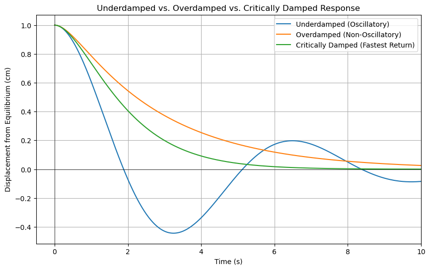
c1 = 0.5 # underdamped
c2 = 3 # overdamped
c3 = 2 * np.sqrt(m*k) # critically damped
# Time vector
t = np.linspace(0, 10, 1000)
# Responses
# Underdamped response
omega_0 = np.sqrt(k/m)
zeta1 = c1 / (2 * np.sqrt(m*k))
omega_d1 = omega_0 * np.sqrt(1 - zeta1**2)
phi = np.arctan(np.sqrt(1 - zeta1**2) / zeta1)
x1 = (1/np.sqrt(1 - zeta1**2)) * np.exp(-zeta1 * omega_0 * t) * np.sin(omega_d1 * t + phi)
# Overdamped response
zeta2 = c2 / (2 * np.sqrt(m*k))
alpha1 = -zeta2 * omega_0 + omega_0 * np.sqrt(zeta2**2 - 1)
alpha2 = -zeta2 * omega_0 - omega_0 * np.sqrt(zeta2**2 - 1)
C1 = alpha2 / (alpha2 - alpha1)
C2 = -alpha1 / (alpha2 - alpha1)
x2 = C1 * np.exp(alpha1 * t) + C2 * np.exp(alpha2 * t)
# Critically damped response
x3 = (1 + omega_0 * t) * np.exp(-omega_0 * t)
# Plotting
plt.figure(figsize=(10, 6))
plt.plot(t, x1, label='Underdamped (Oscillatory)')
plt.plot(t, x2, label='Overdamped (Non-Oscillatory)')
plt.plot(t, x3, label='Critically Damped (Fastest Return)')
plt.axhline(0, color='black',linewidth=0.5)
plt.axvline(0, color='black',linewidth=0.5)
plt.xlabel('Time (s)')
plt.ylabel('Displacement from Equilibrium (cm)')
plt.title('Underdamped vs. Overdamped vs. Critically Damped Response')
plt.grid(True)
plt.legend()
plt.show()
Higher Order Linear
Introduction
Linear Differential Equaiton
We say that a differential equation is linear if it is a linear polynomial in the function and its derivatives. $$a_n(x)y^{(n)}+a_{n-1}(x)y^{(n-1)}+\dots+a_1(x)y'+a_0(x)y=g(x)$$Homogeneous Case
We can call a differential equation homogeoneous if g(x)=0Superposition Principle
If \(y_{1}(x)\) and \(y_{2}(x)\) are two solutions of a homogeneous linear differential equation, then any linear combination \(c_1y_1(x)+c_2y_2(x)\) is also a solution.Characteristic Equation
Let us consider a second order homogeneous linear differential equation $$ay''+by'+cy=0$$ Since the function and its derivatives must cancel each other out, we might guess that the answer is an exponential. $$y=e^{mx}$$ We have the following derivatives for y: $$y'=me^{mx}$$ $$y''=m^2e^{mx}$$ Plugging in to our differential equation: $$am^2e^{mx}+bme^{mx}+ce^{mx}=0$$ $$(am^2+bm+c)e^{mx}=0$$ If the product of two factors is 0, then at least one of the factors must be 0. Because \(e^{mx}\) will never be 0, we need not consider it for finding roots. We can then focus on the equation $$am^2+bm+c=0$$ Which is a simple polynomial of m. We can then find the values of m for which the equation is 0, by factoring, quadratic equation, or completing the square.Let \(m_1\) and \(m_2\) be the roots of the polynomial.
If \(m_1\neq m_2\), we have the following solution $$y=c_1e^{m_1x}+c_2e^{m_2x}$$ If \(m_1=m_2\), or we have repeated roots in the higher order case, the repeats will have an additional factor of x for the number repeat it is. $$y=c_1e^{m_1x}+c_2xe^{m_1x}$$
Complex Roots
But what if we have complex roots?\(e^{mx}\) is still valid for complex m. Euler's formula gives the relationship for a complex exponent. $$e^{ix}=\cos x+i \sin(x)$$ Another relevant formula is that of de Moivre's which states $$(\cos x+i\sin x)^n=\cos nx+i\sin nx$$ The real part of an exponent can be factored out, letting us get $$e^{(a+bi)x}=e^{ax}\left[cos(bx)+i\sin(bx)\right]$$ Since actually do not care whether the constants in front of solutions are real or complex, we get the solutions $$y=e^{ax}\left[c_1\cos(bx)+c_2\sin(bx)\right]$$ as the solution if the root is m=a+bi
Cauchy-Euler Equations
Cauchy-Euler equations are a class of linear differential equations that have variable coefficients. The general form of a Cauchy-Euler equation of order n is given by: $$x^ny^{(n)}+a_{n-1}x^{n-1}y^{(n-1)}+\dots+a_1xy'+a_0y=0$$Characteristic Equation
While we previously assumed an exponential solution for regular homogeneous equations, for Cauchy-Euler equations we assume a solution of the form $$y=x^m$$ Plugging this in gives us the characteristic equation $$m(m-1)(m-2)\dots(m-(n-1))+a_{n-1}m(m-1)\dots(m-2)+\dots+a_0=0$$ We solve the polynomial for m similar to before.Solutions
For distinct real roots, the general solution is $$y(x)=c_1x^{m_1}+\dots+c_nx^{m_n}$$ If a root m is repeated k times, the corresponding terms gain powers of \(\ln(x)\) $$x^m,x^m\ln(x),x^m(\ln(x))^2\dots,x^m(\ln(x))^{k-1}$$ For complex roots \(m=\alpha\pm i\beta\), the corresponding terms in the general solution are $$x^\alpha\cos(\beta\ln(x))\text{ and }x^\alpha\sin(\beta\ln(x))$$Nonhomogeneous
But what if \(g(x)\neq 0\)?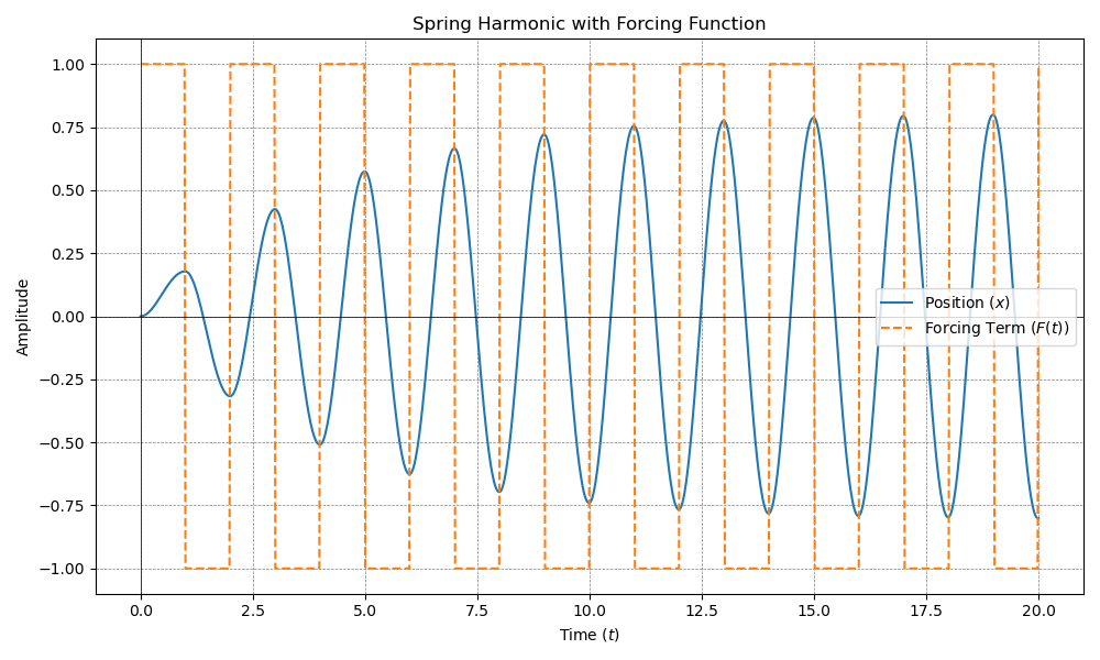
                    import numpy as np
                    from scipy.integrate import odeint
                    import matplotlib.pyplot as plt
                    from scipy.signal import square

                    # Define the system parameters
                    m = 1.0  # Mass
                    b = 0.5  # Damping coefficient
                    k = 10.0  # Spring constant

                    # Define the square wave forcing term
                    A = 1.0  # Amplitude of the square wave
                    f = 0.5  # Frequency of the square wave
                    F = lambda t: A * square(2 * np.pi * f * t)# if (t >= 2 and t <= 8) else 0

                    # Define the ODE system
                    def system(Y, t):
                        x, v = Y
                        dxdt = v
                        dvdt = (F(t) - b * v - k * x) / m
                        return [dxdt, dvdt]

                    # Time array
                    t = np.linspace(0, 20, 1000)

                    # Initial conditions: x = 0, v = 0
                    Y0 = [0, 0]

                    # Solve the ODE
                    solution = odeint(system, Y0, t)

                    # Extract the position (x) from the solution
                    x = solution[:, 0]

                    # Plot the solution
                    plt.figure(figsize=(10,6))
                    plt.plot(t, x, label="Position ($x$)")
                    plt.plot(t, [F(ti) for ti in t], linestyle="--", label="Forcing Term ($F(t)$)")
                    plt.title("Spring Harmonic with Piecewise Forcing Function")
                    plt.xlabel("Time ($t$)")
                    plt.ylabel("Amplitude")
                    plt.axhline(0, color='black',linewidth=0.5)
                    plt.axvline(0, color='black',linewidth=0.5)
                    plt.grid(color = 'gray', linestyle = '--', linewidth = 0.5)
                    plt.legend()
                    plt.tight_layout()
                    plt.savefig("Nonhomogeneous-Spring-Harmonic.png")
                    plt.show()
Method of Undetermined Coefficients
Cases
This can be used when g is a polynomial, exponential, sine, and/or cosine function.Steps
- Guess the form
- Differentiate the guess
- Substitute into the differential equation
- Equate coefficients
Overlaps
If the guessed form is already a solution to the homogeneous version of the differential equation, multiply the guess by a factor of t.Variation of Parameters
Variation of parameters is a more widely applicable method compared to Method of Undetermined Coefficients.Steps
- Determine homogeneous solutions
- Construct Wronskian matrix
- Get coefficients for homogeneous solution
Determine homogeneous solution
Use previous methods to solve the case where g(x)=0Construct Wronskian
For an equation with two homogeneous solutions, the Wronskian is given by: $$W=det\begin{bmatrix} y_1 & y_2\\ y_1' &y_2' \end{bmatrix}$$ This simplifies to \(y_1y_2'-y_2y_1'\)Get Coefficients
The derivatives of the coefficients are given by $$u_1'=\frac{-y_2g(t)}{W}$$ $$u_2'=\frac{y_1g(t)}{W}$$ Upon integrating, this gives the solution $$y_p(t)=u_1(t)y_1(t)+u_2(t)y_2(t)$$Applications
Spring
Exercises
- Solve the Cauchy-Euler equation:
- \(x^2y''+xy'-y=0\)