Laplace Transform

Introduction

The Laplace Transform is a powerful mathematical tool used primarily to simplify the process of analyzing and solving linear ordinary differential equations and systems. By converting functions of time into functions of a complex variable, it transforms differential equations into algebraic equations, which are often easier to solve.

Integral Transform

Definition

For a given function f(t), defined for \(t\geq 0\), The Laplace Transform of f(t) is given by: $$\mathcal{L}\{f(t)\}=F(s)=\int_0^\infty e^{-st}f(t)dt$$ where s is a complex number and F(s) is the image of f(t) under the transform.

Region of Convergence

The Region of Convergence (ROC) is an essential concept associated with the Laplace Transform. It specifies the set of complex numbers, s, for which the Laplace Transform converges.

Inverse Laplace Transform

The Inverse Laplace Transform is a process used to revert a function from the Laplace domain back to the time domain. It is denoted as \(\mathcal{L}^{-1}\)

The mathematical formulation involves complex analysis since you are integrating with respect to a complex variable. Thus, we will just refer to tables when finding the Inverse Laplace Transform.

Definition

If F(s) is the Laplace Transform of a function f(t), then the Inverse Laplace Transform is such that $$f(t)=\mathcal{L}^{-1}\{F(s)\}$$

Properties

Linearity

$$\mathcal{L}\{af(t)+bg(t)\}=aF(s)=bG(s)$$ for constants a,b.

This can be easily shown by the distributive property of multiplication and linearity of integration.

Integration and Differentiation

Frequency Differentiation

$$\mathcal{L}\{tf(t)\}=-F'(s)$$

Frequency Integration

$$\mathcal{L}\{\frac{1}{t}f(t)\}=\int_s^\infty F(s)$$

Time Differentiation

$$\mathcal{L}\{f'(t)\}=sF(s)-f(0)$$

Time Integration

$$\mathcal{L}\{\int_0^tf(t)dt\}=\frac{F(s)}{s}$$

Shifting

Frequency Shifting

$$\mathcal{L}\{e^{at}f(t)\}=-F(s-a)$$

Arguments

Time Scaling

$$\mathcal{L}\{f(at)\}=\frac{1}{a}F(\frac{s}{a})$$

Convolution

The convolution of two functions in the time domain is the pointwise multiplication in the frequency domain. Let h be the convolution of f(t) and g(t): $$h(t)=\int_0^tf(\tau)g(t-\tau)d\tau$$ Then the Laplace transform of h(t) is given by $$\mathcal{L\{h(t)\}}=F(s)G(s)$$

Common transforms

Function \( f(t) \)	Laplace Transform \( F(s) \)
1	\(\frac{1}{s}\) (for \( Re(s) > 0 \))
\( e^{at} \)	\(\frac{1}{s-a}\) (for \( Re(s) > -a \))
\( t^n \) (n>-1)	\(\frac{\Gamma(n+1)}{s^{n+1}}\) (for \( Re(s) > 0 \))
\( e^{at} t^n \)	\(\frac{n!}{(s-a)^{n+1}}\) (for \( Re(s) > -a \))
\( \sin(at) \)	\(\frac{a}{s^2 + a^2}\) (for \( Re(s) > 0 \))
\( \cos(at) \)	\(\frac{s}{s^2 + a^2}\) (for \( Re(s) > 0 \))

Sine in Time Domain and Frequency Domain

The below figure shows a graph of \(f(t)=\sin(2t)\) and its Laplace transform. Note how the max of the Laplace transform is at \(\text{Im}(s)=\pm \omega\)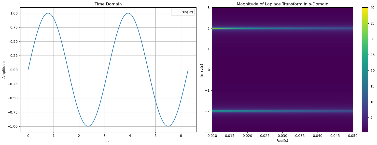

Python Code

Solving ODEs with Laplace Transform

Take Laplace Transform of both sides of the equation

Use a transform table if the functions are common; otherwise, you can explicitly do the integral transform by the definition.

Use algebraic techniques and properties of the Laplace transform to solve for Y(s)

This often involves the use of partial fraction decomposition.

Use the inverse Laplace transform or table to obtain y(t)

Since s is a complex variable, taking an integral with respect to it is non-trivial. Since having complex analysis isn't expected, a transform table should be referred to.

Exercises

1. Compute the Laplace transform of \(f(t)=t^2\)
2. Compute the Laplace transform of \(f(t)=e^{-2t}\)
3. Find the inverse Laplace transform of \(F(s)=\frac{2s+3}{s^2+2s+5}\)
4. Use the laplace transform to solve \(y''+y=\sin(t)\) with initial conditions y(0)=0 and y'(0)=1