Other Figures

import numpy as np
import matplotlib.pyplot as plt

# Define the ODE to be solved (dy/dt = y)
def ode_function(t,y,r,K):
    return r * y * (1 - y / K)

def analytic_solution(t, y0, r, K):
    return K / (1 + ((K - y0) / y0) * np.exp(-r * t))


# Implement the Euler method
def euler_method(t,y, dt,r,K):
    return y + dt * ode_function(t,y,r,K)

# Implement the 4th order Runge-Kutta method
def runge_kutta_method(t, y, dt, r, K):
    k1 = dt * ode_function(t, y, r, K)
    k2 = dt * ode_function(t + 0.5 * dt, y + 0.5 * k1, r, K)
    k3 = dt * ode_function(t + 0.5 * dt, y + 0.5 * k2, r, K)
    k4 = dt * ode_function(t + dt, y + k3, r, K)
    return y + (1/6) * (k1 + 2 * k2 + 2 * k3 + k4)

# Initial conditions
t0 = 0
y0 = 0.1
dt = 5
t_end = 125
r = 0.1
K = 10

# Arrays to store the results
times = np.arange(t0, t_end, dt)
euler_y = [y0]
rk_y = [y0]


# Perform the integration using the Euler method and the Runge-Kutta method
for t in times[1:]:
    euler_y.append(euler_method(t,euler_y[-1], dt,r,K))
    rk_y.append(runge_kutta_method(t,rk_y[-1], dt,r,K))

plt.figure(figsize=(9,6))
analytic_times = np.linspace(t0,t_end,1000)
analytic_y = [analytic_solution(t, y0, r, K) for t in analytic_times]
# Plotting
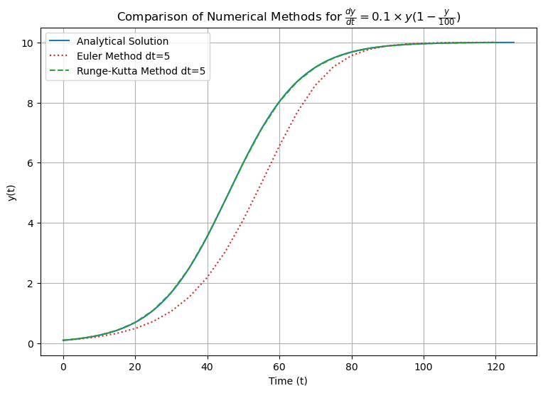
plt.plot(analytic_times, analytic_y, label='Analytical Solution', color='tab:blue')
plt.plot(times, euler_y, label=f'Euler Method dt={dt}', linestyle='dotted', color='tab:red')
plt.plot(times, rk_y, label=f'Runge-Kutta Method dt={dt}', color='tab:green', linestyle='dashed')
plt.xlabel('Time (t)')
plt.ylabel('y(t)')
plt.legend()
plt.title(r'Comparison of Numerical Methods for $\frac{dy}{dt}=0.1\times y(1-\frac{y}{100})$')
plt.grid(True)
plt.show()