Empirical Distribution Function (EDF)

Introduction to Empirical Distributions

While we will talk more on ways to construct and model distributions for variables, we can no longer ignore the topic of statistical testing for goodness-of-fit since it is so important. This pairs with the non-parametric method of the empirical distribution function. This will serve as the most basic method for modeling a distribution.

Recommended Prerequesites

1. Probability
2. Confidence Intervals

Introduction

The Empirical Distribution Function (EDF) is a non-parametric estimator used to approximate the cumulative distribution function (CDF) of a sample. It assigns probability to each observed value in a sample and serves as an essential tool for statistical inference when no assumptions about the underlying distribution are made.

Definition

Given a sample \(\left\{X_1,X_2,\dots,X_n\right\}\), the EDF is defined as: $$F_n(x)=\frac{1}{n}\sum_{i=1}^{n}1_{X_i\leq x}$$ In simple terms, the EDF for a value x is the fraction of the sample that is less than or equal to it. The EDF is a step function that increases by \(\frac{1}{n}\) at each observed data point.

As \(n\rightarrow\infty\), the EDF converges to the true CDF of the population by the Glivenko-Cantelli theorem. Thus, the EDF is a consistent estimator for the CDF.

Empirical Process

Definition

An empirical process captures deviations of the empirical distribution from the true distribution by focusing on the centered and scaled version: $$a_n(x)=\sqrt{n}(F_n(x)-F(x))$$ Here, \(a_n(x)\) represents how much the empirical distribution at point x deviates from the true distribution \(F(x)\), and the scaling factor \(\sqrt{n}\) ensures convergence to a non-degenerate process as \(n\rightarrow\infty\) (Remember that we would have convergence in not scaled by the Glivenko-Cantelli theorem).

Donsker's Theorem

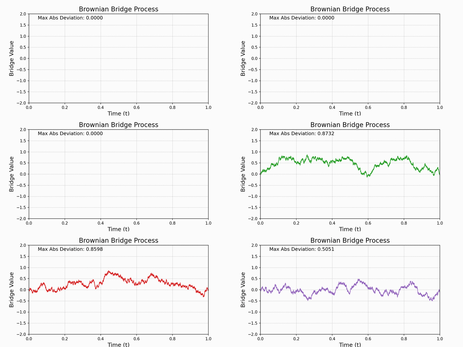
Donkster's Theorem states that an empirical process \(a_n(x)\) converges weakly to a limiting Gaussian process, called the Brownian Bridge.

A Brownian Bridge, \(B(t)\), is a continuous-time stochastic process that starts at zero and returns to zero at the end of the interval, with some properties of a Brownian motion but conditioned to return to zero. The Brownian Bridge is defined over the interval [0,1] as: $$B(t)=W(t)-tW(1)$$ where \(W(t)\) is standard Brownian motion.

Thus; $$a_n(x)\overset{d}{\rightarrow} B(x)=W(F(x))-F(x)W(1)$$

Usage

Also see KS Test Simulator.

Also see 2-Sample KS Test Simulator.

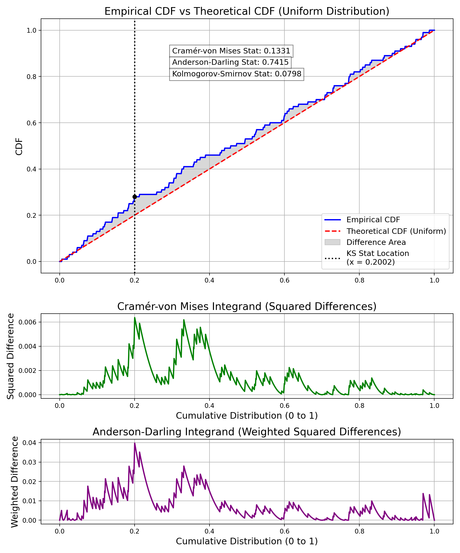
One of the main usages of the EDF and empirical processes is performing goodness-of-fit tests, such as the Kolmogorov-Smirnov (KS) test, where the null hypothesis is that the sample comes from a specified distribution (or in the two-sample case, that two EDFs share a common distribution). The KS test essentially looks at the biggest absolute difference between the EDF and the distribution of the null hypothesis over the whole support. Formally, we write this as: $$D_n=\sup_n\left|F_n(x)-F(x)\right|$$ For a sample, we wouldn't expect zero deviation from the theoretical distribution, but what does the deviation look like under the null hypothesis? Well, at the infimum of the null distribution's support (if it exists), we would expect the EDF would agree with the CDF that $$F_n(L)=F(L)=0$$ where L is the inf of the null distribution's support. If \(F_n(L)>0\) while \(F(L)=0\), that would mean that the support of the true distribution is not the same support as the null distribution, which is a big hint, as you would have been drawing impossible values. But this observation is more relevant for a test like the Anderson-Darling test, which focuses on tails and would be undefined in such a case. By similar logic, let U be the supremum of the distribution if it exists. If \(F_n(U)\lt F(U)=1\), then the sample has values which are too high for the null support.

But let's think of samples where the null hypothesis is true and thus we don't worry about the above. The EDF and the CDF would both be 0 at L and 1 at U, meaning that the absolute difference is 0 for both locations. However, they can vary in the middle. The KS test statistic is asymptotically distributed as the supremum of the absolute value of the Brownian Bridge. The KS test tends to be more sensitive to deviations around the median, but less so at the tails, since the supremum being at the tail would imply a very unlikely sample.

Cramer-von Mises

$$\omega^2=n\int_{-\infty}^{\infty}(F_n(x)-F(x))^2dF(x)$$ The Cramér-von Mises statistic is a distribution-free measure, meaning that its distribution under the null hypothesis is independent from the form of F. It is especially useful for detecting deviations that occur uniformly across the distribution, but it is less sensitive to differences in the tails.

Anderson Darling Distance

The Anderson-Darling distance improves on the Cramér-von Mises statistic by giving more weight to observations in the tails of the distribution, where deviations from the theoretical CDF are often more critical. The Anderson-Darling distance is defined as: $$A^2=n\int_{-\infty}^{\infty}\frac{(F_n(x)-F(x))^2}{F(x)(1-F(x))}dF(x)$$

Confidence Bands

Confidence Bands are analogous to confidence intervals but extend over an entire range of values rather than at a single point. Several methods exist to construct confidence bands for the EDF. The most prominent among them include the Dvoretzky-Kiefer-Wolfowitz (DKW) Inequality, Kolmogorov-Based Bands, and Bootstrap Methods.

DKW Band

The DKW Inequality provides a non-asymptotic, uniform bound on the difference between the EDF and the true CDF. For any \(\varepsilon\gt 0\), the probability that the maximum deviation between \(F_n(x)\) and \(F(x)\) exceeds \(\varepsilon\) is bounded by: $$P(\sup_x\left|F_n(x)-F(x)\right|\gt\varepsilon)\leq 2e^{-2n\varepsilon^2}$$ Thus, to get a \(1-\alpha\) confidence band: Determine episilon: $$2e^{-2n\varepsilon^2}=\alpha$$ $$\varepsilon=\sqrt{\frac{\log(2/\alpha)}{2n}}$$ $$F_n(x)-\varepsilon\leq F(x)\leq F_n(x)+\varepsilon\quad\forall x$$

KS Confidence Band

Since the KS statistic is asymptotically distributed like a Brownian Bridge, we can get a sense by how much things would deviate. $$D_n=\sup_x\left|F_n(x)-F(x)\right|$$ Calculate c based on the Brownian Bridge distribution to get the critical value for \(1-\alpha\). $$\varepsilon=\frac{c}{\sqrt{n}}$$ $$F_n(x)-\varepsilon\leq F(x)\leq F_n(x)+\varepsilon\quad\forall x$$

Empirical Distribution Function Practice Problems

1. Definition of the Empirical Distribution Function (EDF):
   1. Explain what the empirical distribution function (EDF) is. Given a sample dataset \(\{x_1, x_2, \dots, x_n\}\), write down the formula for the EDF, \(F_n(x)\).
   2. For the dataset: \[ \{1.2, 2.3, 2.9, 4.5, 5.1\} \] Calculate the empirical distribution function \(F_n(x)\) at \(x = 3.0\), \(x = 4.5\), and \(x = 6.0\).
2. Glivenko-Cantelli Theorem:
   1. State the Glivenko-Cantelli theorem and explain its significance in the context of empirical distribution functions.
   2. Using the same dataset: \[ \{1.2, 1.5, 2.0, 2.5, 3.0, 4.0, 4.8, 5.5\} \] Simulate 1000 samples from a normal distribution \(N(3, 1^2)\) and compute the maximum difference between the EDF and the true CDF. Plot the EDF and the CDF on the same graph.
3. Kolmogorov-Smirnov Test:
   1. Describe the Kolmogorov-Smirnov (KS) test and its use in comparing an empirical distribution to a theoretical distribution. What is the test statistic for the KS test?
   2. Perform the KS test for the dataset: \[ \{1.3, 2.1, 3.2, 4.5, 5.7, 6.0, 6.3, 7.2\} \] against a theoretical exponential distribution with rate parameter \(\lambda = 0.5\). Compute the KS test statistic and interpret the result.
4. Confidence Bands for the EDF:
   1. What are confidence bands for the EDF? How are they constructed using the Dvoretzky-Kiefer-Wolfowitz (DKW) inequality?
   2. Given the dataset: \[ \{1.0, 1.7, 2.4, 2.8, 3.6, 4.9, 5.0\} \] Construct the \(95\%\) confidence bands for the EDF and plot them alongside the EDF.
5. Applications of the EDF:
   1. Explain how the EDF can be used in non-parametric statistics for hypothesis testing and distribution fitting.
   2. Use the EDF to test whether the following dataset comes from a uniform distribution: \[ \{0.1, 0.3, 0.4, 0.6, 0.8, 0.9, 1.0\} \] Perform a goodness-of-fit test and interpret the results.
6. EDF for Multivariate Data:
   1. Explain how the empirical distribution function can be extended to multivariate data. What are the challenges associated with defining a multivariate EDF?
   2. For the 2D dataset: \[ \{(1.0, 2.0), (2.3, 3.5), (3.1, 4.7), (4.0, 5.0)\} \] Compute the empirical cumulative distribution for each point and plot the results.
7. KS Statistic Distribution
   1. Simulate many samples of at least n=1000 from a distribution and plot a histogram of the KS statistic for each sample. Suggestion: Use a uniform distribution for this.
   2. Simulate many Brownian bridges and record the maximum absolute deviation. Plot it as a histogram.
8. AD Statistic Distribution
   1. Simulate many samples of at least n=1000 from a distribution and plot a histogram of the AD statistic for each sample. Suggestion: Use a uniform distribution for this.
9. CvM Statistic Distribution
   1. Simulate many samples of at least n=1000 from a distribution and plot a histogram of the Cramer-von Mises statistic for each sample. Suggestion: Use a uniform distribution for this.