Introduction to Optimization
Basic Terminology
Recommended Prerequesites
In the last section, we covered parameter estimation strategies. In this section, we will continue coming that, but with a focus on the algorithm and optimization.Fundamentals of Optimization
Optimization is the process of finding the value of a parameter \(\theta\) that results in the maximum or minimum value of the given function \(f(\theta)\).- Maximization: Finding \(\theta\) such that \(f(\theta)\) is as large as possible. This value of \(f(\theta)\) is the maximum and \(\theta\) is called the maximizer.
- Minimization: Finding \(\theta\) such that \(f(\theta)\) is as small as possible. This value of \(f(\theta)\) is the minimum and \(\theta\) is called the minimizer.
Objective Function
An objective function is a mathematical expression that we aim to maximize or minimize with respect to the parameter \(\theta\).Likelihood Function
This measures the probability of observing the given data \(X\) under the parameter \(\theta\). $$L(\theta)=P(X|\theta)$$Example: Bernoulli
Consider a Bernoulli distribution where X can be 1 with probability p or 0 with probability \(1-p\). $$L(p)=\prod_{i=1}^n p^{x_i}(1-p)^{1-x_i}$$Log-Likelihood Function
Often it is more convenient to work in the log-likelihood since the logarithm turns products into sums. $$\ell(\theta)=\log L(\theta)$$Bernoulli Log-Likelihood
$$\ell(p)=\sum_{i=1}^{n}[x_i\log(p)+(1-x_i)\log(1-p)]$$Loss Function
A general term which measures the discrepancy between observed values and those predicted by a model with parameter \(\theta\). One example is the sum of squared residuals (SSR).Analytical Optimization
Analytical optimization involves using calculus.First Derivative Test
The first derivative test looks at points where the first derivative of the function is zero or undefined.- Compute the first derivative \(f'(\theta)\)
- Solve \(f'(\theta)=0\) to find critical points
Second Derivative Test
- If \(f''(\theta)\gt 0\), the function is concave upward, indicating a local minimum
- If \(f''(\theta)\lt 0\), the function is concave downward, indicating a local maximum.
- Compute the second derivative \(f''(\theta)\)
- Evaluate \(f''(\theta)\) at each critical point
Example: MLE for Mean of a Normal
Example: Estimate the mean \(\mu\) of a normal distribution with a known variance \(\sigma^2\), given data \(X=\{x_1,x_2,\dots,x_n\}\). $$L(\mu)=\prod_{i=1}^{n}\frac{1}{2\pi\sigma^2}\exp(-\frac{(x_i-\mu)^2}{2\sigma^2})$$ Taking the log: $$\ell(\mu)=-\frac{n}{2}\log(2\pi\sigma^2)-\frac{1}{2\sigma^2}\sum_{i=1}^{n}(x_i-\mu)^2$$ Computing the first derivative: $$\frac{d\ell}{d\mu}=-\frac{1}{\sigma^2}\sum_{i=1}^{n}(x_i-\mu)(-1)=\frac{1}{\sigma^2}\sum_{i=1}^n(x_i-\mu)$$ Set derivative to zero: $$\frac{d\ell}{d\mu}=0\Longrightarrow \sum_{i=1}^{n}(x_i-\mu)=0$$ $$\mu=\frac{1}{n}\sum_{i=1}^{n}x_i$$ Second derivative test: $$\frac{d^2\ell}{d\mu^2}=-\frac{n}{\sigma^2}\lt 0$$ Since the second derivative is negative, the critical point corresponds to a maximum. $$\hat{\mu}=\bar{x}$$Numerical Optimization Methods
For more complex problems, it is not feasible or possible to get a closed form answer. Numerical Methods use an iterative approach by having an estimate point, taking derivatives there, and then moving the estimate point accordingly.Newton-Raphson Method
The Newton-Raphson uses the first and second derivative to adjust the estimate.- Initial Guess: Choose an initial estimate \(\theta_0\)
- Iteration: \(\theta_{k+1}=\theta_k-\frac{f'(\theta_k)}{f''(\theta_k)}\)
- Convergence Check: If \(|\theta_{k+1}-\theta_k|\lt \varepsilon\), stop; else, repeat
Example: Exponential Distribution
The Exponential distribution has a simple closed form MLE solution, but for pedagogical reasons, we will apply the Newton-Raphson Method to estimate \(\lambda\).Given data \(X=\{x_1,x_2,\dots,x_n\}\) from an exponential distribution, estimate \(\lambda\): $$f(x;\lambda)=\lambda e^{-\lambda x}$$ $$L(\lambda)=\prod_{i=1}^n \lambda e^{-\lambda x_i}=\lambda^n e^{-\lambda \sum x_i}$$ $$\ell(\lambda)=n \log(\lambda)-\lambda\sum_{i=1}^n x_i$$ Now for Newton-Raphson, we have to calculate the first and second derivative: $$\ell'(\lambda)=\frac{n}{\lambda}-\sum x_i$$ $$\ell"(\lambda)=-\frac{n}{\lambda^2}$$ Thus, we get the iteration formula: $$\lambda_{k+1}=\lambda_k-\frac{\ell'(\lambda_k)}{\ell"(\lambda_k)}=\lambda_k-\left(\frac{\frac{n}{\lambda_k}-\sum x_i}{-\frac{n}{\lambda_{k}^2}}\right)$$ This simplifies to $$\lambda_{k+1}=\lambda_k+\left(\frac{n-\lambda_k\sum x_i}{n}\right)$$
Secant Method
The Secant Method is similar to Newton-Raphson but doesn't require computation of the second derivative.Algorithm
- Initial Estimates: Choose two initial guesses \(\theta_0\) and \(\theta_1\)
- Iteration: \(\theta_{k+1}=\theta_k-f'(\theta_k)\left(\frac{\theta_k-\theta_{k-1}}{f'(\theta_k)-f'(\theta_{k-1})}\right)\)
- Convergence Check: If \(\theta_{k+1}-\theta_k|\lt \varepsilon\), stop; else, repeat.
Bisection Method
This technique can be used to find where the derivative is 0 (or more generally a function).Algorithm
- Initial Interval: Choose \([a,b]\) such that \(f(a)\cdot f(b)\lt 0\)
- Compute Midpoint: \(c=\frac{a+b}{2}\)
- Check Sign:
- If \(f(a)\cdot f(c)\lt 0\), set \(b\leftarrow c\)
- Else, set \(a\leftarrow c\)
- Convergence Check: If \(|b-a|\lt \varepsilon\), stop; else repeat
Gamma Distribution Example
The Gamma distribution is a continuous probility distribution whose PDF is given by: $$f(x;\alpha,\beta)=\frac{x^{\alpha-1}e^{-x/\beta}}{\beta^{\alpha}\Gamma(\alpha)}$$ where- \(x\in(0,\infty)\)
- \(\alpha\) is the shape parameter \((\alpha\gt 0)\)
- \(beta\) is the scale parameter \((\beta\gt 0)\)
- \(\Gamma(\cdot)\) is the gamma function
Log-Likelihood
Given a sample of n independent observations \(\{x_i\}\) from a Gamma distribution with known \(\beta\) and unknown \(\alpha\), the log-likelihood function is: $$\ell(\alpha)=(\alpha-1)\sum_{i=1}^{n}\log(x_i)-\frac{\sum_{i=1}^{n}x_i}{\beta}-n\alpha\log(\beta)-n\log(\Gamma(\alpha))$$ To find the MLE of \(\alpha\), we need to solve \(\ell'(\alpha)=0\), where \(\ell'(\alpha)\) is the first derivative of the log-likelihood function with respect to \(\alpha\), also known as the score function.$$S(\alpha)=\frac{d\ell}{d\alpha}=\sum_{i=1}^{n}\log(x_i)-n\log(\beta)-n\psi(\alpha)$$ where \(\psi(\dot)\) is the digamma function For Newton's Method, we need the second derivative of the likelihood function (first derivative of score function) calculated as well: $$S'(\alpha)=\frac{d^2\ell}{d\alpha^2}=-n\psi^{(1)}(\alpha)$$ where \(\psi^{(1)}(\alpha)\) is the trigamma function.
Newton Example
Our iterative equation in Newton's Method will be: $$\alpha_{n+1}=\alpha_n-\frac{f(\alpha_n)}{f'(\alpha_n)}$$ In the context of MLE, we set \(f(\alpha)=S(\alpha)\) and \(f'(\alpha)=S'(\alpha)\) to find where \(S(\alpha)=0\).Import Libraries
import numpy as np
from scipy.special import psi, polygamma  # Digamma and trigamma functions
Defining the Functions
def neg_log_likelihood(alpha, data, beta):
    n = len(data)
    if alpha <= 0:
        return np.inf  # Shape parameter must be positive
    sum_ln_x = np.sum(np.log(data))
    sum_x = np.sum(data)
    ll = (alpha - 1) * sum_ln_x - n * alpha * np.log(beta) - n * np.log(np.math.gamma(alpha)) - sum_x / beta
    return -ll  # Negative log-likelihood

def score_function(alpha, data, beta):
    if alpha <= 0:
        return np.inf
    n = len(data)
    mean_ln_x = np.mean(np.log(data))
    score = n * (mean_ln_x - np.log(beta) - psi(alpha))
    return score

def score_function_derivative(alpha, data, beta):
    if alpha <= 0:
        return np.inf
    n = len(data)
    derivative = -n * polygamma(1, alpha)  # polygamma(1, alpha) is the trigamma function
    return derivative
Problem Set-Up
# True parameters
alpha_true = 5.0  # Shape parameter
beta_known = 2.0  # Known scale parameter

# Generate sample data
np.random.seed(0)
sample_size = 1000
data = np.random.gamma(shape=alpha_true, scale=beta_known, size=sample_size)
Implementation
# Initial guess
alpha_initial = 1.0

def newton_raphson(f, f_prime, x0, args=(), tol=1e-6, max_iter=100):
    alpha = x0
    for i in range(max_iter):
        f_val = f(alpha, *args)
        f_prime_val = f_prime(alpha, *args)
        if np.isnan(f_val) or np.isnan(f_prime_val) or f_prime_val == 0:
            raise ValueError("Invalid function value or derivative encountered.")
        alpha_new = alpha - f_val / f_prime_val
        if alpha_new <= 0:
            alpha_new = alpha / 2  # Ensure alpha remains positive
        if abs(alpha_new - alpha) < tol:
            print(f"Converged in {i+1} iterations.")
            return alpha_new
        alpha = alpha_new
    raise ValueError("Maximum iterations reached without convergence.")

# Run Newton-Raphson method
alpha_estimated = newton_raphson(score_function, score_function_derivative,
 x0=alpha_initial, args=(data, beta_known))
print(f"Estimated alpha (Newton-Raphson Method): {alpha_estimated:.4f}")
Secant Method
$$\alpha_{n+1}=\alpha_{n}-f(\alpha_n)\times\frac{\alpha_n-\alpha_{n-1}}{f(\alpha_n)-f(\alpha_{n-1})}$$ where \(f(\cdot)=S(\alpha)\).Defining the Functions
def neg_log_likelihood(alpha, data, beta):
    n = len(data)
    if alpha <= 0:
        return np.inf  # Shape parameter must be positive
    sum_ln_x = np.sum(np.log(data))
    sum_x = np.sum(data)
    ll = (alpha - 1) * sum_ln_x - n * alpha * np.log(beta) - n
    \* np.log(np.math.gamma(alpha)) - sum_x / beta
    return -ll  # Negative log-likelihood

def score_function(alpha, data, beta):
    if alpha <= 0:
        return np.inf
    n = len(data)
    mean_ln_x = np.mean(np.log(data))
    score = n * (mean_ln_x - np.log(beta) - psi(alpha))
    return score
Initialize
# Initial guesses
alpha0 = 1.0
alpha1 = 10.0
Implementation
def secant_method(f, x0, x1, args=(), tol=1e-6, max_iter=100):
    alpha_prev, alpha = x0, x1
    for i in range(max_iter):
        f_prev = f(alpha_prev, *args)
        f_curr = f(alpha, *args)
        if np.isnan(f_prev) or np.isnan(f_curr) or (f_curr - f_prev) == 0:
            raise ValueError("Invalid function values or zero denominator encountered.")
        alpha_new = alpha - f_curr * (alpha - alpha_prev) / (f_curr - f_prev)
        if alpha_new <= 0:
            alpha_new = (alpha + alpha_prev) / 2  # Ensure alpha remains positive
        if abs(alpha_new - alpha) < tol:
            print(f"Converged in {i+1} iterations.")
            return alpha_new
        alpha_prev, alpha = alpha, alpha_new
    raise ValueError("Maximum iterations reached without convergence.")

alpha_estimated_secant = secant_method(score_function, x0=alpha0, x1=alpha1,
 args=(data, beta_known))
print(f"Estimated alpha (Secant Method): {alpha_estimated_secant:.4f}")
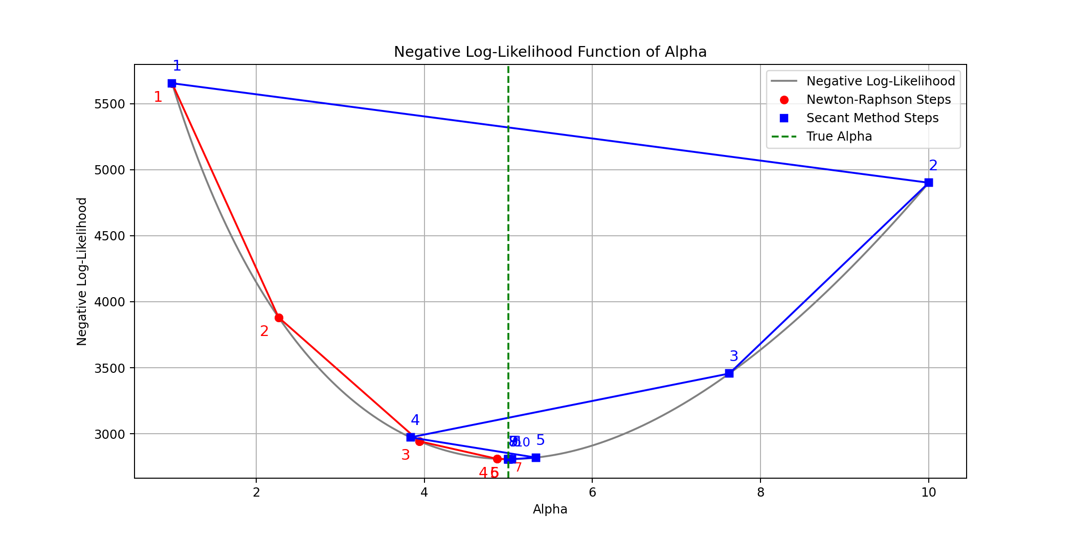
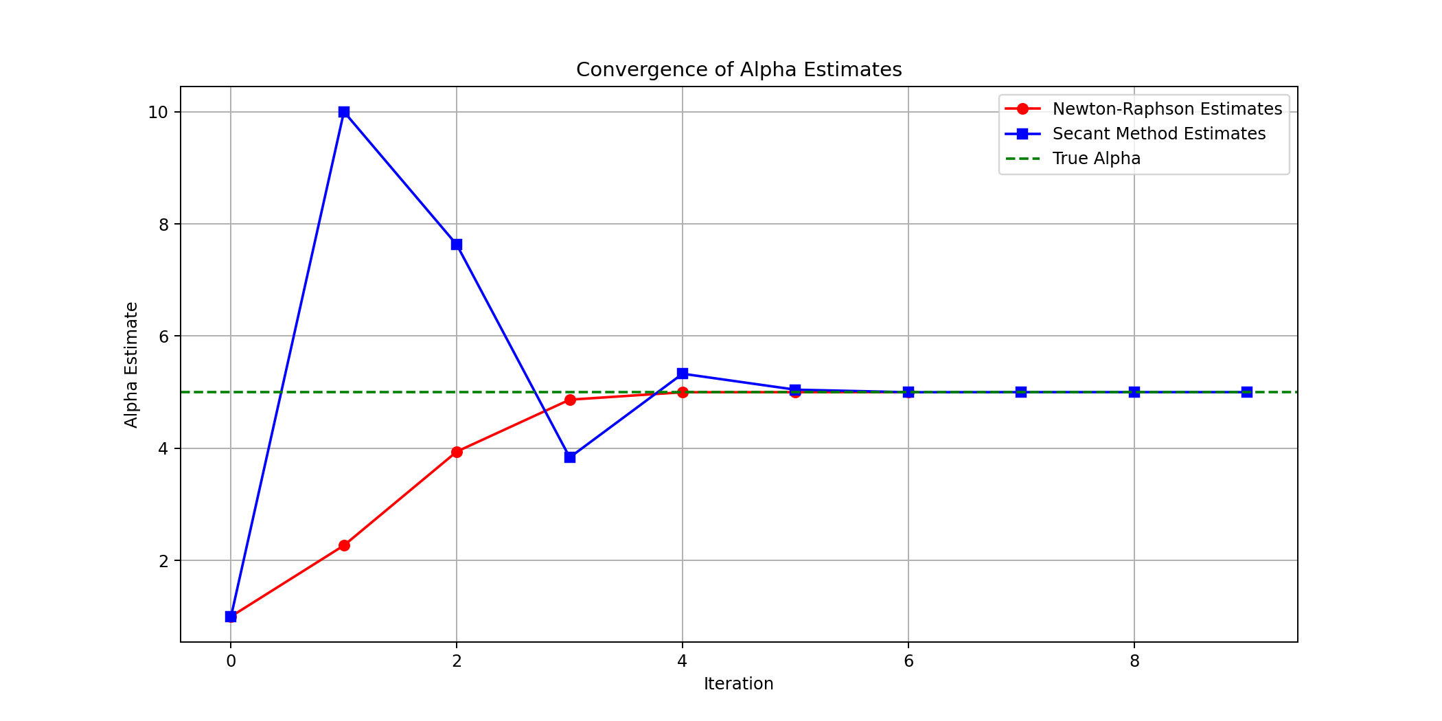
Comparison


Optimization Practice Problems
-
Solve for the root of the function \( f(x) = x^2 - 4 \) using the secant method.
- Use initial guesses \( x_0 = 1.5 \) and \( x_1 = 2.5 \).
- Perform 3 iterations and approximate the root to 4 decimal places.
-
Minimize the function \( f(x) = (x - 3)^2 + 4 \) using the secant method.
- Use initial guesses \( x_0 = 1 \) and \( x_1 = 5 \)
- Perform 3 iterations to approximate the minimum to 4 decimal places.
-
Minimize the function \( f(x) = x^3 - 3x^2 + 2x \).
- Apply the secant method starting with \( x_0 = 0 \) and \( x_1 = 2 \).
- Perform 4 iterations and determine the approximate value of \( x \) at the minimum.
-
For \( f(x) = \ln(x) + x^2 - 2x \), find the minimum using the secant method.
- Start with \( x_0 = 0.5 \) and \( x_1 = 1.5 \).
- Perform 3 iterations. Does the method converge? Why or why not?
-
Minimize the function \( f(x) = x^4 - 4x^3 + 6x^2 - 4x \) using Newton's method.
- Use \( x_0 = 2.5 \) as the initial guess.
- Perform 3 iterations and approximate the minimum to 4 decimal places.
-
The function \( f(x) = \sin(x) + x^2/2 \) has a minimum near \( x = -1 \).
- Apply Newton's method with the initial guess \( x_0 = -1 \).
- Perform 3 iterations to approximate the minimum to 4 decimal places.